Graphics Reference
In-Depth Information
Figure 15.17 shows the results of this shader.
In the left-hand image,
uMin
and
uMax
are set to
show all data values. Because you are looking at
everything, some key parts of the volume might be
obscured. It would then be very helpful if you cull
away the values you really have no interest in. In
the right-hand image, the low (blue) values have
been culled, giving us a much beter view of the
shape of the middle-to-high values.
This same shader can be modified to pro-
duce isosurfaces as well. An isosurface is the locus
of points corresponding to a specific scalar value
in the volume, referred to as S*. All you have to
do is change the volume rendering fragment shader to consider, in its march
through the volume, only the first scalar value that is within a certain tolerance
of S*. An example of this is shown in Figure 15.18. The actual code to do this is
left as an exercise. (You knew that was coming, right?)
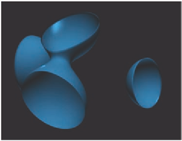
Figure 15.18.
Isosurface.
More on Transfer Functions
The mapping of a scalar value to its color was introduced in Chapter 8. This
mapping was glossed over in the shaders that we discussed earlier in this
chapter with the call to the
Rainbow( )
routine. We should now look closer
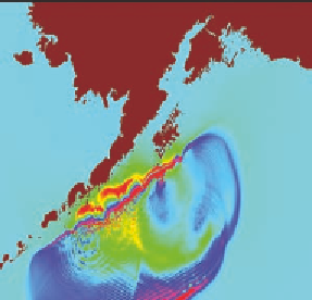
Figure 15.19.
Two different transfer functions applied to tsunami data of the coast of the
Aleutian Peninsula in Alaska. (Image courtesy of Chris Janik.)