Graphics Reference
In-Depth Information
Notice the use of the
Rainbow( )
function. This sets
up the transfer function that defines the mapping between
each scalar value and its assigned color. Routines like this
are often writen to accept a normalized input, in this case
the variable called
t
. The value of
t
is
0
when the scalar value
is a minimum and 1 when it is a maximum. In this way,
the color mapping routine does not need to know anything
about the nature of the scalar values. We cover transfer func-
tions in more detail later in this chapter.
Also notice the use of the uniform variables
uMin
and
uMax
in the fragment shader. They are assigned by sliders
in the
glman
user interface, and are used to cull the display
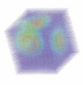
based on data values. In the image in Figure 15.9, the small-
est values in the dataset have been culled.
This isn't a visualization book, but as we discuss visualization shaders,
we need to talk about some fundamental visualization concepts. A disadvan-
tage of the uniform point cloud is that it can create severe display artifacts.
In orthographic projection mode, sometimes the dots line up, creating the
“row of corn problem.” In perspective projection mode, the alignment creates
annoying (but often interesting) Moiré paterns. These two kinds of artifact are
shown in Figure 15.10.
What can you do to avoid these artifacts? A common answer is to use a
different type of point cloud, known as a
jiter cloud
. In a jiter cloud, the dots
are randomly shifted by small amounts in
x
,
y
, and
z
, and the data values
Figure 15.9.
Culling dots based on
scalar value.
Figure 15.10.
Artifacts in uniform point clouds; the “row of corn” problem, left, and Moiré
paterns (right).