Graphics Reference
In-Depth Information
want to blend both images. There are a number of different common kinds of
blends. In the sections below, we will sketch a few of them and show examples.
It should be straightforward for you to complete any implementations that we
do not give completely. In addition, we have included a few more blends as
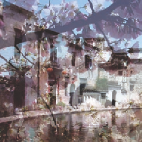
chapter exercises. Figure 11.25 shows two sample images that we will use to
illustrate many of the blending operations we discuss.
Other Combinations
Complex and interesting interpolations of two images are possible because
you can use any function that takes two RGB color values and returns another
RGB color value. The function could act on entire RGB vectors or it could act
on the individual color components separately. We explore a few of these
below, and there are a few more in the exercises.
Cosine Interpolation
As an example, consider a cosine-based interpolation from [20] that looks
interesting; Figure 11.26 shows the effect. The same pixel from both images is
read, and the color components of the two pixels are com-
bined, using cosine multipliers. The cosine is applied to
each component, so components nearer one are increased.
If we take
Argb
as the color of the “after” image and
Brgb
as
the color of the “before” image, as above, then the blended
color is given by
color
(
)
−∗ ∗
(
)
=−∗
ρα π
cos*
Argb
β
cos
π
Brgb
where
ρ
is a base color, basically an overall luminance, and
α
and
β
are chosen to weight the two images (and either
ραβ
++ cannot exceed 1 or you must clamp the result).
Sample fragment shader code for this operation is
given below. Notice that we have used values of 0.5 and
-0.25 as the base value and cosine multiplier, respectively;
in an exercise, we encourage you to experiment with these
(and we suggest that you use
glman
uniform slider variables to do so).
Figure 11.26.
The cosine interpola-
tion of the two sample images.
const float PI = 3.14159265;
uniform sampler2D uBeforeUnit, uAfterUnit;
in vec2 vST;