Graphics Reference
In-Depth Information
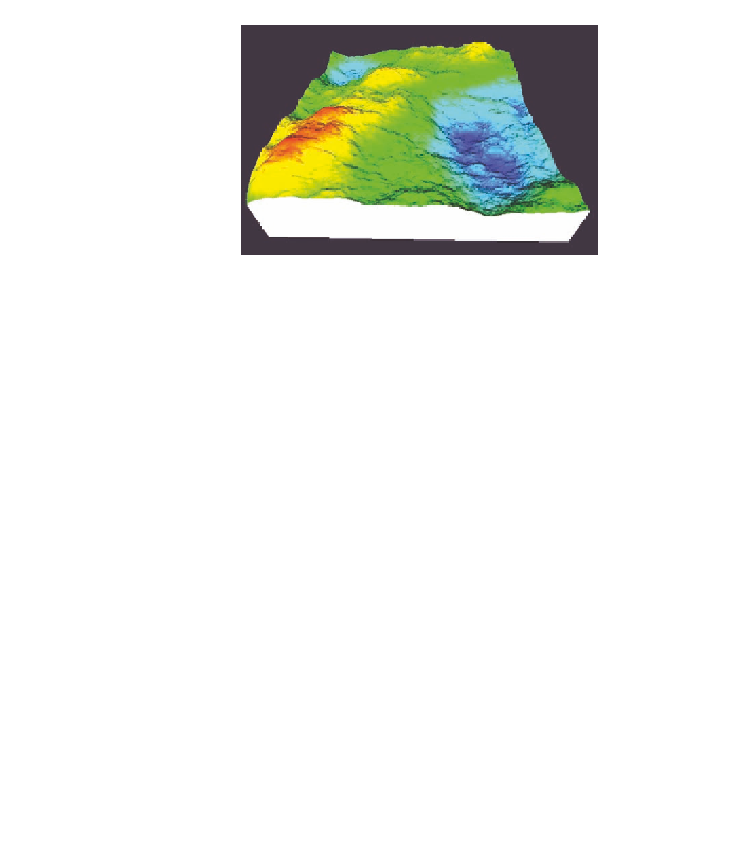
Figure 10.6.
Four octaves of 2D noise represented as a pseudocolored height field.
the 2D image that you saw in the simple 1D noise graphs: the four-octave noise
has the same general shape, but much more high-frequency variation. (The
noise is quintic value+gradient type.) The appearance is that the higher-octave
noise has more detail and is consequently visually richer. Figure 10.6 shows a
4-octave 2D noise function represented as a height field.
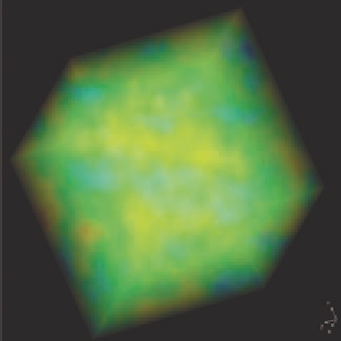
When we look at 3D noise, we have
a litle more diicult visualization prob-
lem. A 3D noise function is visualized as
a pseudocolored volume in Figure 10.7.
Even without seeing specific interior
details, you can still see that there is
some familiar-looking variation in color
within the cube.
We could look at this in several
ways, including explorations through
some standard visualization techniques,
as shown in Figure 10.8. This shows an
isosurface with its isovalue equal to the
midrange value of the 3D noise, and we
can easily see the greatly increased com-
plexity that comes with the additional
octaves of noise.
Figure 10.7.
Three-dimensional one-
octave noise viewed as pseudocolor in
a direct volume rendering.