Graphics Reference
In-Depth Information
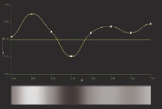
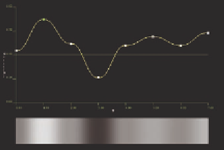
Figure 10.3.
Forcing the gradients to zero (left) and computing the gradients from the dis-
tribution of points (Catmull-Rom, right). Notice how much more natural the curve appears
as it passes through the connections when a reasonable slope is computed instead of artifi-
cially set to zero.
That is, to get the parametric slope at noise point
i
, draw a vector from the
previous point to the next point, and take half of it. Figure 10.3 shows how this
changes the overall shape of the noise curve, making it a lot smoother.
Since all four coefficients are spelled out above, you now have the full
cubic polynomial functions for any combinations of values and gradients you
want in a noise function. Using the same conditions for
t
= 1 at the end of one
segment and
t
= 0 at the beginning of the next segment will ensure that the
functions are differentiable at the point between them, giving you an overall
C
1
noise function.
What about
quintic
noise functions? Here we need to place additional
conditions on the function at the given points in order to derive the six coef-
ficients on the general quintic polynomial function
2
3
4
5
Nt ABtCt t t t
()
=+++++
.
We already have the function value
N
and the gradient
G
at each point,
giving us four conditions. The two additional necessary conditions are given
by specifying the curvature
C
of the function at the points. The curvature is
given by the second derivative, so we now have three expressions to evaluate.
Besides the
N
(
t
) function above, we have
dN
dt
B t t t t
Gt
()
==++ +
23 4
2
3
+
5
4
,
dN
dt
2
2
Ft
3
.
Ct
()
=
= ++ +
2612
C t t
20
2