Graphics Programs Reference
In-Depth Information
“Particles” button - “Emission” tab, you see that 1000 parti-
cles are being generated starting at frame 1, ending at frame
200, with a lifetime of 50 frames. You will also see “Ran-
dom” and “Even Distribution” boxes ticked so the particles
are being spread between the faces in a random order as
they are generated. “Random” would appear to take prece-
dence over “Even Distribution.” Note also that “Jittered” is
highlighted in blue—“Jittered” means that particles appear
in a random position in any one face on the object. Untick
the “Random” box and play the animation. The particles
are now generated from one face after the other around the
circle plane object. Increase the “Lifetime” value to 200 to
make the particles display longer in the animation. Note
that if the animation is played without the object selected,
the particles will appear as small black dots instead of the
little orange squares.
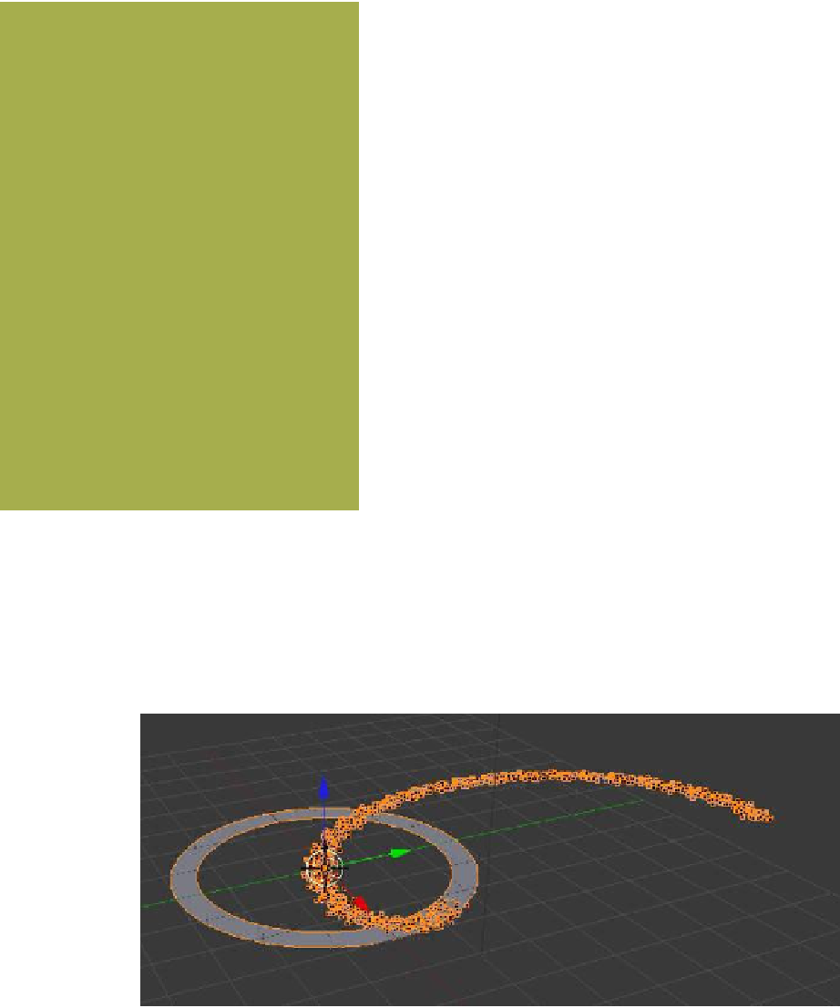
Cycling the animation in the timeline to frame 200 pro-
duces a spiral array in the 3D window, which may be ren-
dered as an image (Figure 13.17). You will however have to
relocate the camera in the scene to render an image of the
complete spiral. By default, Blender renders an image of a
particle system that includes the emitter object. To render
without the emitter object, go to the “Render” tab in the
“Particles” button and untick the “Emitter” box.
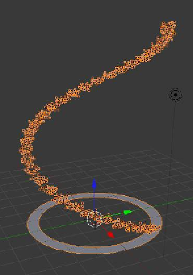
The spiral has been generated with a “Normal Velocity”
value of 1.000. If this value is deleted and the “Emitter Object Y” value in the “Velocity” tab
is set to 1.000, the spiral will generate flat along the
y
-axis when the animation is replayed
(Figure 13.18)—how the array of particles is generated is controlled by the values entered
in the “Velocity” tab.
So far, the particles that have been generated have been displayed as dots or little orange
squares in the 3D window and have been rendered as halos. In the “Render” tab, you will
Figure 13.17
Figure 13.18