Information Technology Reference
In-Depth Information
1
0.9
0.8
0.7
0.6
_
A/A
0
0.5
simulations
0.4
0.02
0.2
0.4
0.3
smooth maximum
0.02
0.2
0.4
0.2
sharp maximum
0.1
0.02
0.2
0.4
0
0.01
0.1
1
10
100
a
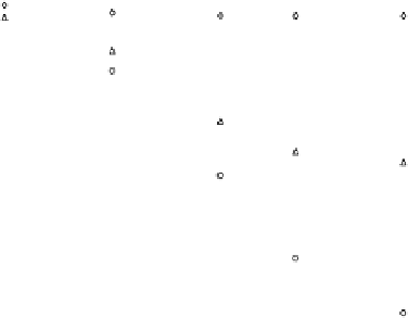
Fig. 15.6. Average tness
h
A
i
=A
0
versus the coecient a, of the tness function, Eq. (15.19),
for some values of the mutation rate . Legend: numerical solution corresponds to the numerical
solution of Eq. (15.17), smooth maximum refers to Eq. (15.21) and sharp maximum to Eq. (15.25).
neglecting last term, and substituting q(u) = A(u)p(u) in Eq. (15.17) we get:
hAi
A
0
= 12
for u = 0
(15.25)
and
(hAiA(u)1 + 2)
q(u1)
q(u) =
for u > 0 :
(15.26)
Near u = 0, combining Eq. (15.25), Eq. (15.26) and Eq. (15.19), we have
q(u) =
(12)au
2
q(u1) :
In this approximation the solution is
u
12a
1
(u!)
2
;
q(u) =
and
u
1
u!
2
:
We have checked the validity of these approximations by solving numerically
Eq. (15.17); the comparisons are shown in Fig. (15.6). We observe that the smooth
maximum approximation agrees with the numerics for small values of a, when A(u)
varies slowly with u, while the sharp maximum approximation agrees with the
numerical results for large values of a, when small variations of u correspond to
large variations of A(u).
y(u) = A(u)q(u)'
1
A
0
A
0
hAia
(1 + au
2
)