Information Technology Reference
In-Depth Information
a
b
1
V
V(s)
f
V
r
0
0
T
s
0
1
t
c
d
1
V
−
V( )
s
0
V( )+
−
s
−
t
e
0
V(s)
f
t
−
H ( )
V
r
0
0
T
s
0
1
s
0
t =s / T
t
0
0
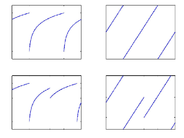
Fig. 13.2. Dynamics of membrane potentials and phases. Upper panels show free evolution of
potential (a) and corresponding phase (b). Lower panels show evolution of potential (c) and phase
(d) with an inhibitory spike arriving at time s
0
. (Modied from [81].)
where g(:) > 0 species the local dynamics of neuron j, "
ji
denotes the strength
of synaptic coupling from neuron i to neuron j, and s
i
species the time neuron i
sends its mth spike. When a neuron i reaches a potential threshold V
i
((s
i
)
) = V
,
its potential is reset to V
i
(s
i
) = V
r
and it sends a spike which is received by the
postsynaptic neurons j after a delay time
v
> 0. Here, K(:) is a response kernel
that determines the post-synaptic current in response to an incoming spike signal.
Such a kernel satises
R
1
1
K(s)ds = 1 and K(s) = 0 for s < 0. Often one considers
the limiting case of fast synaptic response, K(s) = (s). For such systems the
smooth dynamics of the neurons is interrupted by two kinds of events that occur
at discrete times only: sending of spikes (and reset) and receiving of spikes. This
results in a hybrid dynamical system [13, 19, 133] with continuous-time dynamics
interrupted at discrete times where maps are applied [10, 23].
A universal representation of the network dynamics provides elegant analyti-
cal access to state space trajectories. The network of spiking neurons (13.1) with
K(s) = (s) is equivalently described by the dynamics of phase variables
i
(t)1
with rescaled time variable t = s=T : The free solution V (s) of Eq (13.1) in the
absence of coupling (all "
ji
= 0) through the initial condition V (0) = V
r
increases
monotonically and is assumed to reach the threshold after a time T such that
V (T
) = V
. This free solution denes a bijective map (Fig. 13.2a,b)
U : (
; 1]!(V
; V
]; 7! U() := V (T ) ;
(13.2)