Geography Reference
In-Depth Information
where
q
0
.
for
r
≤
b
q
=
0
for
r > b
It is easily verified that the solution of (6.28) satisfying the requirement of
continuity in
and ∂
∂r at r
=
b is
f
0
q
0
b
2
/2
r
2
/6
−
−
≤
for r
b
=
(6.29)
f
0
q
0
b
3
/ (3r)
−
for r>b
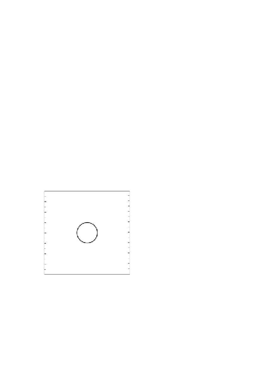
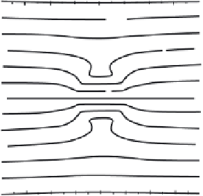
Figure 6.10 shows the pattern of potential temperature and geostrophic wind
induced by this compact positive potential vorticity anomaly. The distribution of the
θ surfaces indicates that static stability is enhanced in the ball of positive potential
vorticity and is reduced both above and below the ball. Because potential vorticity
is conserved (and has zero anomaly outside the ball), positive vorticity anomalies
are induced above and below the ball of potential vorticity to compensate the
reduced stability, and hence the geostrophic flow induced by the potential vorticity
anomaly extends well beyond the boundary of the anomaly.
6.3.4
Vertical Coupling Through Potential Vorticity
As illustrated above, a potential vorticity anomaly at one level yields a nonzero
geopotential anomaly (and hence nonzero geostrophic winds) at other levels. This
4
4
320
3
3
2
312
2
0
312
0
1
1
-8
8
304
0
0
296
296
-1
-1
288
288
-2
-2
-3
-4
-3
-4
280
(a)
(b)
-4
-3
-2
-1
-0
1
2
3
4
-4
-3
-2
-1
-0
1
2
3
4
Fig. 6.10
Vertical cross sections showing potential temperature (left) and geostrophic wind (right)
induced by a ball of constant potential vorticity of nondimensional radius unity. A constant
standard atmosphere potential vorticity is added to the anomaly induced by the ball of
potential vorticity. (Right) Solid contours indicate flow into the page and dashed contours
indicate flow out of the page. The horizontal and scaled vertical distances are normalized by
the radius of the potential vorticity ball. For a ball of 250-km radius the horizontal distance
shown is 2000 km and the vertical distance is 20 km (assuming that the buoyancy frequency
is 100 times the Coriolis frequency). (Adapted from Thorpe and Bishop, 1995)