Multiple Comparison Procedures - Analysis of Variance Designs - page 145

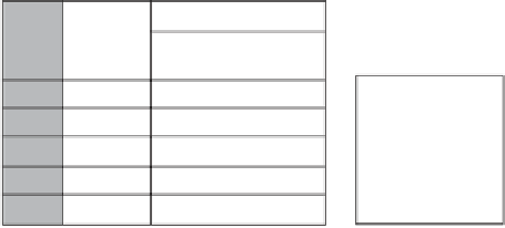
The GLM Procedure
Least Squares Means
Adjustment for Multiple Comparisons: Dunnett

H0:LSMean = Control

satscore
LSMEAN group Pr > ⏐ t ⏐

This is the probability of
the mean difference
between Group 0 and
Group 2 occurring by
chance alone. This
probability is less than
our alpha level and is
therefore statistically
significant.

0
2
4
6
8

412.857143
474.285714
552.857143
614.285714
622.857143

0.0128
< .0001

< .0001

< .0001

Figure 7.19 The output from the Dunnett comparisons.

drawn to the a posteriori pairwise comparisons available as post hoc
tests.

7.21 POLYNOMIAL CONTRASTS (TREND ANALYSIS)
7.21.1 POLYNOMIAL FUNCTIONS
As you may remember from your high school algebra class, variables can
be raised to a power. For example, in the expression x 2 , 2 is the exponent
of x ; we say that the variable x is raised to the second power (it is squared).
In simplified form, a polynomial is a sum of such expressions where the
exponents are whole positive numbers.
Part of the naming conventions for polynomials is to identify them
by the highest appearing exponent appearing in the function. Thus, if
the highest exponent is 2, we would label it as quadratic , if the highest
exponent is 3 we would label it as cubic , and if the highest exponent is 4
we would label it as quartic .

7.21.2 THE SHAPE OF THE FUNCTIONS
We require for a trend analysis that the levels of the quantitative inde-
pendent variable approximate interval measurement. If they do meet this
requirement, then the shape of the function is interpretable. This is because
the spacing of the groups variable on the x axis is not arbitrary and thus
the shape of the function is meaningful; if the independent variable did
not approach interval measurement, using equal spacing is completely
arbitrary (it is appropriate only aesthetically), and the shape of the func-
tion is not meaningful since different spacing of the groups along the axis
would alter the shape of the function.
Table 7.4 presents some information about examples of polynomial
functions on the assumption that the groups on the x axis are spaced on
an equal interval basis. Linear functions are straight lines. To draw such
a function, all you need to do is to connect two data points (the means
of two groups). In the function shown in Table 7.4, x is raised to the first
power. Figures 7.20A and B show linear functions.