Inversion Strategy - Models and Methods of Magnetotellurics - page 481

Its inversion is focused on estimating the resistivity of the upper crust. The TS-3
model, obtained from the

−

inversion, was used as a starting model. Here we fixed
all resistivities except for crustal blocks that contact the sedimentary cover. The

⊥ −

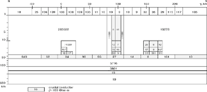
⊥ − and inversion resulted in the TS-4 model, shown in Fig. 12.24. It confirms the

galvanic connection between the vertical conductive zone B and sediments, and
reveals the asymmetry of the highly resistive upper crust whose resistivity changes
from 283 000 Ohm

· m in the north to 13 000 Ohm · m in the south (in the initial TS

model, from 100 000 Ohm m in the south).

The TS-4 model is the final model obtained from the successively applied auto-
matic partial inversions. Its agreement with the initial TS model is evident. All of the
essential TS structures are well resolved in the TS-4 model. Misfits between these
models at the overwhelming majority of sites do not exceed 0.02 in tippers and 2.5 ◦
in phases. The transverse apparent-resistivity misfits are shown in Fig. 12.25. The
TS-4 and TS models yield similar regional variation in

· m in the north to 10 000 Ohm ·

⊥ with a local scatter caused
by geoelectric noise. Note that irregular alternation of cells with higher and lower
resitivity within zones B and C as well as within the crustal condutive layer can be
readily smoothed without increasing the model misfits.
Next we consider the case when the a priory information on the media bordering
the profile is rather scanty. In that event we have to apply the adjustment method sug-
gested in Sect. 10.1.1. Figure 12.26 presents the longitudinal

−

curves obtained

=− = −

at the edges of profile, y 50 km and y 200 km, as well as the average ¯

curve that is taken as a curve for the normal apparent resistivity

N . One-dimensional
inversion of this curve yields a normal background which is introduced symmetri-
cally into the interpretation model from Fig. 12.19 at a distance of 300 km from
each edge of the profile. Repeating the partial inversions in the same succession as in
case of an asymmetrical normal background, we obtain a final model TS-5 shown in
Fig. 12.27. All of the essential TS structures are clearly seen in this model. The only
essential difference between models constructed with asymmetric and symmetric

⊥ ad impedance phases ⊥ has Fig. 12.24 Model TS-4; inversion of the apparent resistivities

been performed using the blocky II2DC program; resistivity values in Ohm · m are shown within

blocks; blocks of lower crustal resistivities are shaded (cf. Fig. 12.16)