The Interpretation Model - Models and Methods of Magnetotellurics - page 378

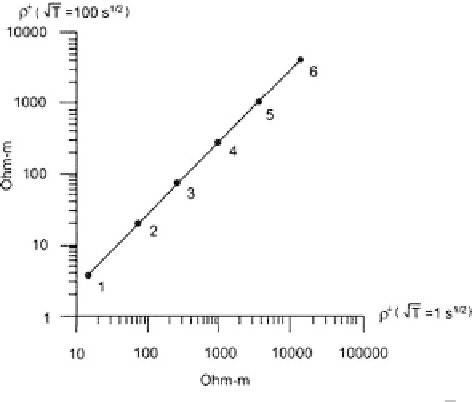
⊥ ( √ T ⊥ ( √ T 100 s 1 / 2 )and 1s 1 / 2 ) Fig. 11.3 Correlation between the apparent resistivites = =

⊥ -curves obtained in the model of the S- effect related to descending and ascending branches of the

shown in Fig. 11.1; 1, 2, 3 ... - observation sites

in the sediments conductance S 1 do not exceed 10%. The peculiarity of this case
is that not only the descending low-frequency branches of the ⊥ -curves, but their

ascending high-frequency branches also are shifted vertically from the locally nor-
mal

⊥ -curves suffer the static distortion over the
entire frequency range including the ascending and descending branches, which
carry information on the upper layer and substratum. Note that within this frequency
range the

n -curves. One can see that the

⊥ -curves are not distorted being closely related to the locally normal

n -
curves (Fig. 11.8). Using the phase indication, that is, marking a boundary between
zones with diverged and converged phase curves, we evaluate the initial period of
the

0.25 s (Fig. 11.9). Let us give a glance at Fig. 11.10 correlating
the descending and ascending branches of the

-effect as T s ≈

⊥ -curves. The graph can be approx-
imated by a straight line with inclination close to 45 ◦ . Remarkable as it is, the

−
effect demonstrates the same relations between descending and ascending branches
of the ⊥ -curves as the strong S − effect.

The above definitions of the S − and − effects retain their meaning in the three-

dimensional situation. An example of the effect caused by a three-dimensional

outcropped inhomogeneity with random lognormal distribution of resistivities is
given in Figs. 11.11 and 11.12. Here the apparent-resistivity curves,

−

xy and
yx , with their high-frequency ascending branch and low-frequency two-humped
descending branch are conformally scattered about the normal

N -curve. Their static
shift embraces 2.5 decades, whereas the corresponding phase curves, xy and yx ,

merge with normal N -curve. Correlating the descending and ascending branches

curves, we get a graph with inclination close to 45 ◦ , which
indicates the strong static shift (Fig. 11.13).
Behind the S

of the xy − and yx −

− −

effects are the same physical mechanisms. However, they
operate in different frequency intervals and on different spatial scales - so, these

and