The Interpretation Model - Models and Methods of Magnetotellurics - page 377

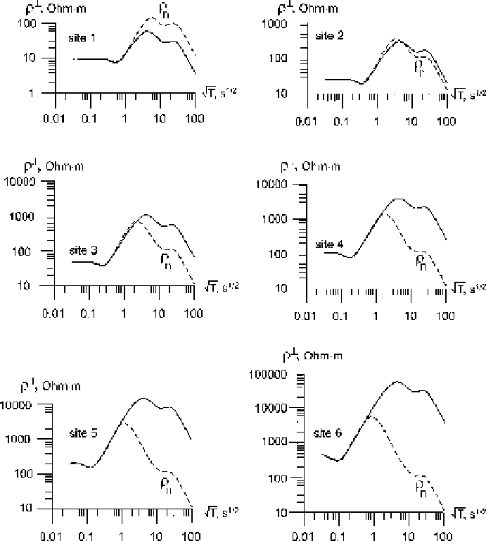
Fig. 11.2 Transverse apparent-resistivity curves in the model of the S- effect from Fig. 11.1

⊥ -curves diverge within a range of the slightly distorted
high-frequency branches of the

Fig. 11.5. The adjacent

⊥ -curves, but they come together within a range of
the statically shifted low-frequency branches of these curves. So, the initial period
T s of the S -effect can be evaluated as a boundary between zones with diverged and
converged phase curves. Using this indication in the case under consideration, we
get T s ≈

9s.
Now consider the effect. The case is illustrated in Fig. 11.6. Here the upper

layer contains a two-dimensional small outcropped inclusion, 10 m thick and 120 m
wide, consisting of conductive and resistive sections, while the host medium is the
same as in the previous model given in Fig. 11.1. The transverse

−

⊥ -curves are
presented in Fig. 11.7. They show the conspicuous static shift, though variations