Information Technology Reference
In-Depth Information
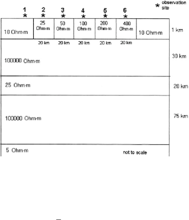
Fig. 11.1
Two-dimensional model of the
S-
effect
to descending and ascending branches of the
⊥
-curves. The graph is plotted to
bilogarithmic scale. It is approximated
by
a straight line with i
nc
lination close to
45
◦
. Thus, a relationship between
⊥
(
√
T
⊥
(
√
T
100 s
1
/
2
) and
1s
1
/
2
) can be
=
=
represented as
⊥
(
√
T
⊥
(
√
T
100 s
1
/
2
)
1s
1
/
2
)
=
≈
C
=
(11
.
1)
⊥
(
√
T
⊥
(
√
T
=
100 s
1
/
2
)
≈
+
=
1s
1
/
2
)
,
log
log
C
log
where
C
is a constant. This relation indicates a strong
S
effect (due to high resis-
tivity of the substratum underlying the inhomogeneous upper layer). It is easy to
verify that a decrease in the substratum resistivity weakens the
S
−
−
effect and this
manifests itself in diminishing the regression inclination.
The transverse phase curves are exhibited in Fig. 11.4. Their high-frequency
ascending
and
low-frequency
descending
branches
are
close
to
the
locally-
normal
n
-curves being slightly distorted. However, in the middle-frequency
range they depart from the locally normal
n
-curves and this distortion amounts
up to 50
◦
.
It is important to find the initial period
T
s
of the static shift (a period separating
the distorted descending branch of the
⊥
-curves from their undistorted ascend-
ing branch). A good indicator can be given by the phase curves. Have a look at