Information Technology Reference
In-Depth Information
Using the spline approximation, the values
Z
brd
are extrapolated in such a way that
the condition
Z
brd
=
Z
brd
is valid on a new boundary contour
C
1
and the derivative
of
Z
brd
along the normal to
C
1
vanishes. Given these conditions, we assume that
the impedance
Z
brd
is close to the normal impedance
Z
N
of a horizontally layered
medium in the infinite normalized area
S
N
external with respect to
C
1
and determine
its normal conductivity
N
(
z
) by the one-dimensional inversion of the impedances
Z
brd
. At the last stage we perform the one-dimensional inversion of the impedances
Z
brd
extrapolated in the transition zone
S
t
and find gently varying transition conduc-
tivities
z
) between the observation area
S
0
and the normalized area
S
N
. So,
we get a model, in which a normal background and a transition zone embrace the
observation area:
t
(
x
,
y
,
⎧
⎨
(
x
,
y
,
z
)
M
∈
S
0
(
M
)
=
t
(
x
,
y
,
z
)
M
∈
S
t
(10
.
4)
⎩
N
(
z
)
M
∈
S
N
.
The conductivity
t
in the transition zone can be corrected at the stage of the three-
dimensional inversion.
Likewise, the normal background is introduced using the effective impedances
Z
eff
.
To test this algorithm, we should make sure that an expansion of the transition
zone
S
t
has no significant effect on the results of MT and MV inversions in the
central part of the observation area
S
0
.
The adjustment method based on the averaging and extrapolation of
Z
brd
,
Z
eff
or
Z
,
Z
⊥
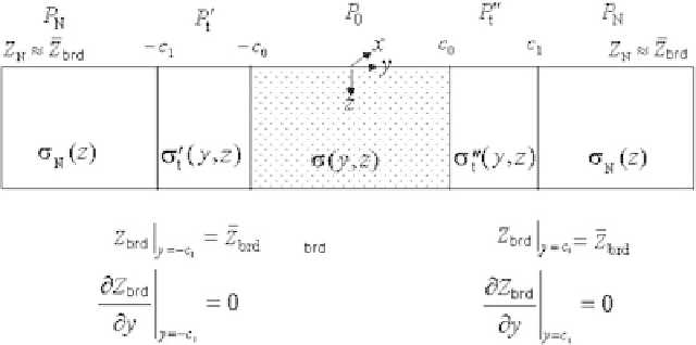
can be applied in a 2D approximation of elongated structures. Let observa-
tions be carried out along a transverse profile
P
0
from
y
=−
=
c
0
(Fig. 10.2).
The average of the invariant
Z
brd
at the edges of the profile is determined as
c
0
to
y
Fig. 10.2
Introduction of a normal background into the 2D interpretation model