Information Technology Reference
In-Depth Information
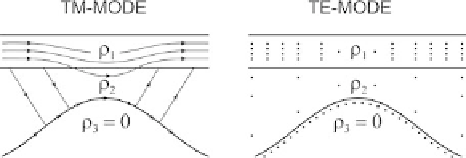
Fig. 8.21
TM- and TE-mechanisms of the electromagnetic distortions caused by the astheno-
sphere relief
⊥
,
calculated
for different periods
L
are presented in Table 8.2. We see that in the TM-mode the
asthenosphere topography is severely screened over a wide range of periods
L
up to
500 km (
⊥
,
along with galvanic and inductive ratios
distortion factors
⊥
≤
,
⊥
≤
23), whereas in the TE-mode the asthenosphere topog-
raphy manifests itself quite distinctly even at
L
0
.
38
2
.
=
,
=
96).
One can say that the TE-mode may be more sensitive to the asthenosphere topogra-
phy than the TM-mode.
=
100 km (
0
.
73
1
.
8.2.2 Magnetotelluric Anomalies Caused
by the Asthenosphere Uplift
Now we turn to more realistic model discribing a single two-dimensional uplift of
the asthenosphere (Fig. 8.22). Here the layers
3
simulate the conductive
sediments, the resistive lithosphere, and the conductive asthenosphere, while
1
,
2
and
v
and
h
are the half-width of the uplift and its amplitude.
Let us begin with a model of the uplift. Its parameters are:
1
=
10 Ohm
·
m
,
h
2
=
h
1
=
1km
,
2
=
10000 Ohm
·
m
,
h
2
=
99 km
,
3
=
10 Ohm
·
m
,v
=
250 km
,
50 km.
Figure 8.23 presents the field profiles, which pass across the asthenosphere uplift
in the
y
−
direction. The electric and magnetic fields, normalized to the normal fields
E
N
x
E
N
y
H
N
y
, are calculated for periods relating to the descend-
ing branch of the apparent-resistivity curves. The asthenosphere uplift manifests
itself in minima of the electric fields. Once again we see the distinction between
the TM- and TE-modes. In the TM-mode we have the transverse field
E
y
with
,
,
given at
|
y
| →∞
Table 8.2
Distortion factors
a
⊥
,
a
in relation to the period
L
L, km
100
200
300
500
1000
2000
TM-mode
⊥
0.45
0.9
1.34
2.23
4.46
8.93
a
⊥
0.0001
0.03
0.14
0.38
0.69
0.87
TE-mode
1.96
3.92
5.88
9.8
19.6
39.2
a
0.73
0.87
0.92
0.96
0.98
0.99