Information Technology Reference
In-Depth Information
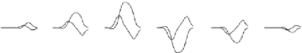
Fig. 7.40
Tipper curves, Re
W
zy
and Im
W
zy
, outside and over the horst in the model shown in
Fig. 7.38;
y
-distance to the centre of the model
l
=
15
,
75
,
150
,
300 km;
v
=
15km
,
l
=
30
,
150
,
300
,
600 km;
v
=
30 km
,
l
=
60
and
l
are the width and length of the horst.
Straightforward computation testifies that on this parametrical set the horst elon-
gation
e
,
300
,
600
,
1200 km, where 2
v
may be well used as a stable indicator of quasi-two-dimensionality.
By way of example consider a horst 60 km wide and 60 km long (
e
=
l
/
2
v
=
1).
=∞
Figure 7.43 demonstrates the three-dimensional and two-dimensional (
e
)
apparent-resistivity, impedance-phase and tipper curves, obtained along a central
profile running in the
y
direction.
The apparent resistivity
−
xy
,
yx
and phase
xy
,
yx
curves observed over
the horst (
y
=
0
,
y
=
22
.
5 km) show up rather strong flow-around effect.
(2D),
(2D)
Here,
at
low
frequencies,
we
get
xy
(3D)
>>
xy
(3D)
>>
⊥
(2D). The flow-around effect also man-
ifests itself in the tipper curves Re
W
zy
(3D) and Im
W
zy
(3D), measured out-
side
⊥
(2D),
and
yx
(3D)
<<
yx
(3D)
<<
5 km). But it quickly attenuates as the horst elonga-
tion
e
increases. Figure 7.44 demonstrates the apparent resistivity, impedance-
phase and tipper curves for a horst 60 km wide and 600 km long (
e
the horst
(
y
=
37
.
=
10).
Here
the
curves
for
xy
(3D)
,
yx
(3D)
and
xy
(3D)
,
yx
(3D)
virtually
merge
(2D)
,
⊥
(2D) and
(2D)
,
⊥
(2D), while
with the two-dimensional curves for
the curves for Re
W
zy
(3D)
,
Im
W
zy
(3D) are sufficiently close to the curves for
Re
W
zy
(2D)
10 provides the quasi-two-
dimensionality of the horst 60 km wide. The same condition is found for the horsts
15 and 30 km wide. It should be recognized that this condition is valid not only over
the horst, but in its visinity
,
Im
W
zy
(2D). It seems that the condition
e
≥
5
l
as well.
Now compare the quasi-two-dimensionality condition, obtained in the horst
model, with conditions, obtained in the elliptic-cylinder model with equivalent
contrast of conductances:
m
|
y
| −
v
≤
0
.
S
1
/
S
1
=
=
(
h
1
−
h
)
/
h
1
=
0
.
3
.
Using estimates
given by (7.132) for the 10%-difference between
A
(3D) and
A
(2D), we get
e
xy
≥
.
,
e
yx
≥
.
2inthe
S
1
−
interval and
e
xy
≥
.
,
e
yx
≥
.
10
3
21
13
7
43
3inthe
−
h
interval. Consider the quasi-two-dimensionality conditions for the horst and
elliptic-cylinder. They are almost the same for the longitudinal
xy
−
curves (
e
≥
10
against
e
xy
≥
10
.
3
,
e
xy
≥
13
.
7) and considerably differ for the transverse