Information Technology Reference
In-Depth Information
3
d
, we set coth(
d
)
1 and receive the same estimates (7.70) for the
S
-effect as in the two-segment model:
If
v
≥
v/
≈
⎧
⎨
S
1
S
1
⎧
⎨
n
S
1
S
1
Z
N
|
| =
v
+
˙
|
y
| =
v
+
0
y
0
Z
⊥
(
Z
N
S
1
S
1
⊥
(
±
v
)
≈
±
v
)
≈
⎩
⎩
n
S
1
S
1
¨
|
y
| =
v
−
0
.
|
y
| =
v
−
0
(7
.
82)
Moving away from the central segment, the
S
-effect exponentially attenuates.
We can turn to Table 7.1 and estimate a distance, at which
⊥
approaches its locally
normal value ˙
n
with an accuracy of 5%. It is a question of several adjustment
distances.
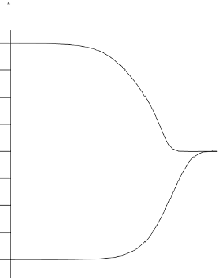
It would be interesting to estimate the width
w
=
2
v
of the central segment, at
⊥
is close to its locally
whose middle (
y
=
0) the transverse apparent resistivity
n
. Figure 7.17 shows the dependence of
⊥
(0)
/
w
normal value ¨
¨
N
on
for models
with and
S
1
/
S
1
100 km and
S
1
/
S
1
=
.
,
d
=
=
,
d
=
0
01
100
1000 km. The
ρ
(0)
ρ
n
10000
1000
S
‛‛
1
S
1
= 0.01
100
‛‛
=
100
km
d
10
1
0.1
S
‛‛
1
= 100
0.01
‛
1
S
d
‛‛
=
1000
km
0.001
0.0001
w, km
0.01
0.1
1
10
100
1000
10000
⊥
(0)
Fig. 7.17
The
w
-dependence of the normalized transverse apparent resistivity
/
¨
n
obtained
in the middle of the central segment of the model shown in Fig. 7.16