Models of the Near-Surface Distortions - Models and Methods of Magnetotellurics - page 223

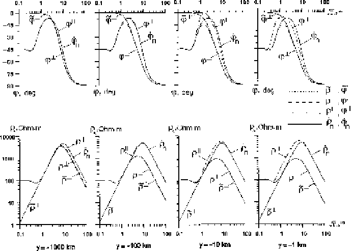
Fig. 7.10 Longitudinal and transverse apparent-resistivity and impedance-phase curves over the
left conductive segment in the model shown in Fig. 7.9; y -distance to the boundary between seg-
ments; ˜ ⊥ , ⊥ -analytical solution, ⊥ , ⊥ and , -numerical solution by means of the finite ˜

1 , 1 element method, ˙ n , n - locally normal solution. Model parameters: ˙ = 10 Ohm · m =

10 5 100 Ohm · m , h 1 = 1km , 2 = Ohm · m , h 2 = 99 km , 3 = 0

Figures 7.10 and 7.11 show the apparent-resistivity and impedance-phase curves
obtained over the left and right segments at different distances from the con-
ductance discontinuity.
First of all note that within the ⊥ -curves

plotted from the analytical and numerical solutions agree fairly well. The ascending
branches of the

S 1 - and h -intervals the transverse

⊥ -curves are not distorted. They coincide with ascending branches
of the locally normal ⊥ -curves

n -curves. However, the descending branches of the

are distorted by the S -effect. They are shifted from the locally normal n -curves,

down over the left conductive segment and up over the right resistive segment. The
maximum S -effect is observed at the boundary between the segments. With distance
from the conductance discontinuity the S -effect monotonously decreases. It vanishes
at y 3000 km over the left segment ( d

≈− = 1000 km) and at y ≈ 1200 km

over the right segment ( d

316 km). These estimates are in a good agreement
with Table 7.1. Now have a look at the transverse phase curves. In passing to the
h -interval the

=

⊥ -curves, plotted from the analytical and numerical solutions, merge
together and with lowering frequency they approach the locally normal n -curves.

A remarkable property of the S -effect is that the drastically shifted branches of the
⊥ -curves correspond to the slightly distorted branches of the

⊥ -curves.