Information Technology Reference
In-Depth Information
ωμ
0
h
2
S
1
|
G
|
2
1.0
6
4
2
0.1
6
4
2
50
λ
1
/
h
1
=
100
25
(y
-
y
′
)/h
-1.2
-0.8
-0.4
0
0.4
0.8
1.2
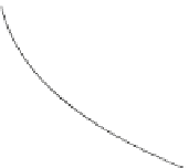
Fig. 7.8
The Green function in the Tikhonov-Dmitriev model, the TE-mode; model parameters:
h
2
/
h
1
=
49
,
2
=∞
,
3
=
0; curve parameter:
λ
1
/
h
1
Summing up, we define the longitudinal impedance
⎧
⎨
q
(
y
,
)
q
(
y
,
)
Z
n
(
y
)
=
in the
S
1
-interval
S
1
(
y
)
Z
(
y
)
≈
(7
.
51)
⎩
q
(
y
,
)
Z
n
(
y
)
=−
iq
(
y
,
)
0
h
in the
h
-interval
,
q
(
y
,
)
→
1as
→
0
where
q
(
y
) is a frequency-dependent complex factor accounting for distortions
caused by the inductive interaction between near-surface excess currents.
The longitudinal apparent resistivities and phases assume the form
,
⎧
⎨
)
o
S
1
(
y
)
(
y
,
(
y
,
)
n
(
y
)
=
in the
S
1
-interval
(
y
)
≈
(7
.
52)
⎩
(
y
,
)
n
(
y
)
=
(
y
,
)
o
h
2
in the
h
-interval
|
q
(
y
,
)
|→
1as
→
0
⎧
⎨
n
(
y
)
+
arg
q
(
y
,
) n e
S
1
-interval
(
y
)
≈
(7
.
53)
n
(
y
)
+
arg
q
(
y
,
)
in the
h
-interval
,
⎩
arg
q
(
y
,
)
→
0as
→
0
2
where
.
Thus, the induction effects are most pronounced within the
S
1
-interval. They
may tangibly affect the ascending branches of the apparent-resistivity and phase
curves, and their one-dimensional inversion may give false geoelectric structures.
But within the
h
-interval the induction effects die out and the one-dimensional
(
y
,
)
= |
q
(
y
,
)
|