Abrupt Climate Changes During the Holocene Across North America From Pollen and Paleolimnological Records - Abrupt Climate Change: Mechanisms, Patterns, and Impacts - page 177

Comparisons in the frequency domain provide a useful
strategy for analyzing possible causes of the variability at
any time scale; however, there is interest in direct compari-
son of individual transitions to determine leads and lags in
the climate system as well as to describe the nature of the
transition (Figure 4). Comparing the various series, there are
similarities but also differences among them, and it is diffi-

large distances can lead to dif culties. In any geophysical

series, any individual climate transition may be missing, due
to local factors such as sedimentation hiatus or simply a lack
of local response to the climate forcing. Therefore, oscilla-
tions may appear shorter or longer in some records but not
even be seen in others, and this may explain, in part, the
differences between records. The interactions between slow
variations and more abrupt changes further complicates the
interpretation of Holocene climate records, especially during
the mid-Holocene, when scale interactions between the
orbital and suborbital scales seems to have reduced the
millennial-scale climate variability [Fisher, 1982; Gajewski,
1983]. An individual paleoclimate series records only the
regional climate, but it is the spatial pattern of climate that is
the response to forcing [Gajewski, 1987; Viau et al., 2006],
and a suf

-
cult to propose an overall spatial model of Holocene climate
variability using these data. For example, the North Ameri-
can mean July temperature anomaly, Santa Barbara, and
West African marine records all show major changes at
around 8, 6, and 3.2 ka, but these transitions are not as clear
in the other records. Higher-frequency changes are not al-
ways coherent. This is due in part to the low density of sites
with high enough temporal resolution and also due to issues
with dating the sediments. As noted by Viau et al. [2006] and
Gajewski et al. [2007], “ wiggle-matching ” series from across

ciently dense series of sites is needed to under-
stand changes in the general circulation.

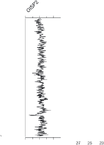
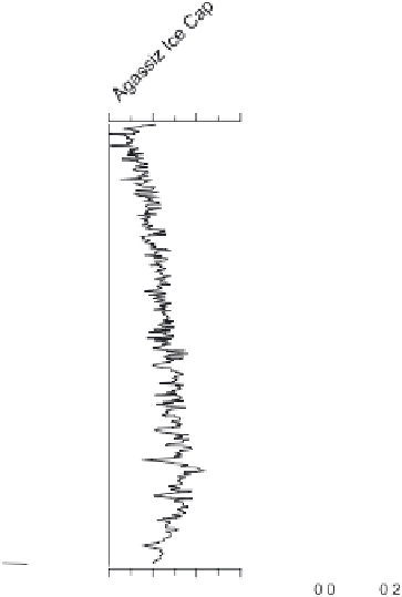
Figure 4. Several high-resolution paleoclimate series from North America and adjacent regions: (a) North Atlantic benthic
δ

13 C[Oppo et al., 2003]; (b)

“ stacked ” record of hematite-stained glass, an ice-rafted detritus record from Bond et al.

18 O record from the Agassiz Ice Cap,
Ellesmere Island [Fisher et al., 1995]; (e) mean July temperature for North America, reconstructed using pollen data [Viau
et al., 2006]; (f )

18 O record from the GISP2 ice core, Greenland [Alley et al., 1997]; (d)

[2001]; (c)

δ δ

18 O for the Santa Barbara Basin [Fridell et al., 2003]; and (g) warm season sea surface temperatures off
the West African coast [deMenocal et al., 2000]. Shading delimits the four major periods in the North American pollen-
based July temperature anomaly reconstruction.

δ