Visualizing Relationships - Data Points: Visualization That Means Something - page 199

y-coordinates, and the actual text to print—you have all of these. Like
the bubbles, the x is murders and the y is burglaries. The actual labels
are state names, which is the first column in your data frame.
text(crime$murder, crime$burglary, crime$state, cex=0.5)
The cex argument controls text size, which is 1 by default. Values greater
than one can make the labels bigger and the opposite for less than one. The
labels can center on the x- and y-coordinates, as shown in Figure 6-20.
At this point, you don't need to make a ton of changes to get your graphic
to look like the final one in Figure 6-15. Save the chart you made in R as a
PDF, and open it in your favorite illustration software to refine the graphic
to what you want it to look and read like. You can thin the axis lines and
remove the surrounding box to simplify a bit. You can also move around
some of the labels, particularly in the bottom left, so that you can actu-
ally read the state names; then bring the bubble for Georgia to the front—
before it was hidden by the larger Texas bubble.
There you go. Type in ?symbols in R for more plotting options. Go wild.
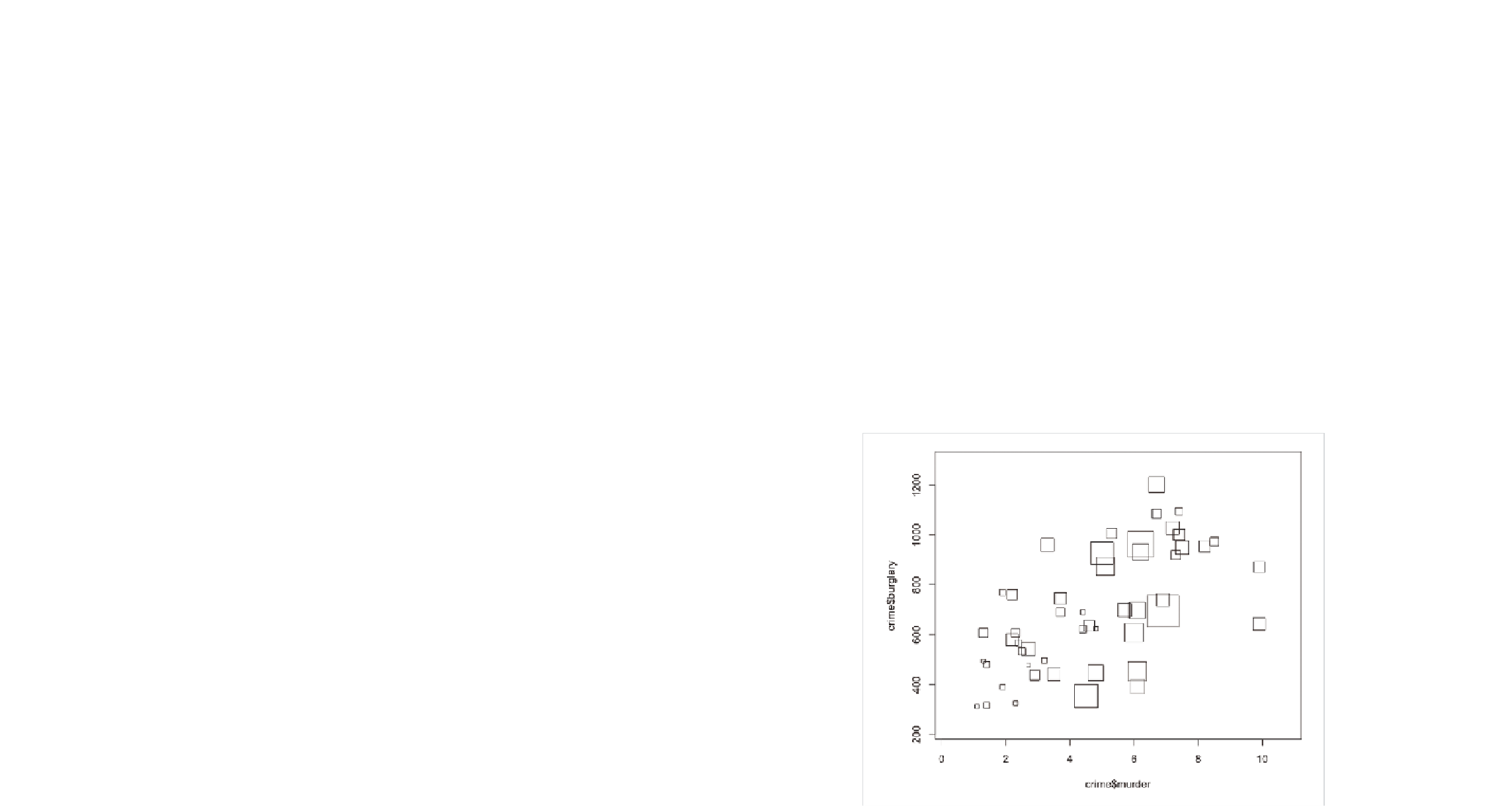
FIGurE 6-19 Using squares instead of circles