Study on the Monolithic Muffler Acoustic Field Performance of the Train Air-Conditioning - Advanced Research on Computer Education, Simulation and Modeling - page 141

∂ p ∂

ρ

2

= c

∂ t ∂

(3)

Acoustic wave equation

uv

uv uv

∂
∇=− ∂

1

2

p

2

p

2 2

ct

(4)

2.2 The Sub-grid Model of the Acoustic Fields

Because SYSNIOSE pre-treatment functions are weak, we should create a finite
element model of the muffler at the proportion of 1:1 in ANSYS, and create two ducts
model whose length both are125mm at the opening and the entrance of the finite
element model. We also mesh the model according to "each wave length with 6 units"
rule after modeling in ANSYS:

c

= Δ (5)
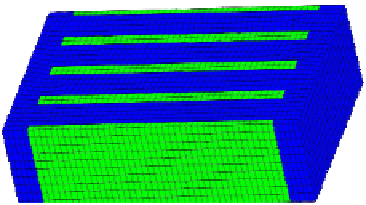
The highest frequency we analysis and calculate is 4322Hz. Figure 1 shows the
finite element model after the model is imported into the SYSNIOSE.

f

max

6L

Fig. 1. Mesh model after imported into the NIOSE

2.3 Boundary Conditions and Material Properties Setup of the Acoustic Field
Model

After the model is imported into the SYSNIOSE, we should define boundary
conditions and material properties, and the boundary conditions of the acoustic field
include in the inlet, outlet and wall settings. Table 1 is boundary conditions, Material
properties setup is as follow: Fluid density is 1.225 kg/m 3 , Sound wave velocity is
340 m /s, Impedance is 12000pa.s/m 2 , the structure coefficient is 4, Porosity is 0.4.

Table 1. Boundary conditions setup

3RVLWLRQ %RXQGDU\ %RXQGDU\W\SHV W\SHV 9DOXH DOXH

,QOHW 8QLW VSHHG

2XWOHW $OO VRXQGDEVRUELQJ H[SRUW

0XIIOHU ZDOO 5LJLG ZDOO 'HIDXOW