Geoscience Reference
In-Depth Information
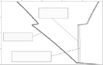
Figure 3.3
Simplified
daytime profiles of humidity
and temperature through the
atmospheric boundary layer
(both shown as thick black
lines) and the associated
potential temperature and
virtual potential temperature
calculated from these two.
Potential temperature is
shown as a thin black line and
the virtual potential
temperature as a gray line.
Mixing ratio (g kg
−
1
)
7.5
Temperature (K)
0.0
2.5
5.0
250
260
270
280
290
300
60
60
Potential
temperature
70
70
80
80
Temperature
90
90
Virtual potential
temperature
100
100
Virtual potential temperature
As well as correcting for the influence of the hydrostatic pressure gradient on
temperature, it is also possible to make a simple correction for the additional
effect of changes in water vapor content on local atmospheric density
(buoyancy) by calculating
q
v
, the
virtual potential temperature
at any level.
This is done using a definition analogous to Equation (3.16) but expressed in
terms of the virtual temperature as defined by Equation (2.14). Virtual
potential temperature is therefore defined relative to the virtual temperature,
T
v
=
T
(1
+
0.61
q
), by:
R
c
a
p
100
⎛
⎞
θ
=
T
(3.18)
⎜
⎟
v
⎝
P
⎠
To a good approximation, the vertical gradient of virtual potential temperature
can be calculated from that for virtual temperature using:
∂
θ
∂
=
T
v
v
Γ
d
∂
z
∂
z
(3.19)
Figure 3.3 shows the calculated profiles of potential temperature and virtual
potential temperature for simple example gradients of temperature and humid-
ity. Note that in well-mixed portions of the atmospheric boundary layer (ABL),
the vertical gradients of humidity and potential temperature (but
not
actual
temperature) are often small. During the day a reversal in potential temperature
often then separates this well-mixed layer from the atmosphere above where
the air is typically drier than in the ABL. Although the actual temperature of
this overlying air may decrease with height, it typically falls at a rate less than