Geoscience Reference
In-Depth Information
1.5
0.05
0.18
0.05
0.30
1.0
0.18
0.43
0.30
0.68
0.43
0.93
0.55
1.05
0.68
0.5
1.18
0.76
0.05
0.18
0.30
0.40
0
12
18
0
6
12
18
0
6
Day 1
Day 2
Day 3
Time (hours)
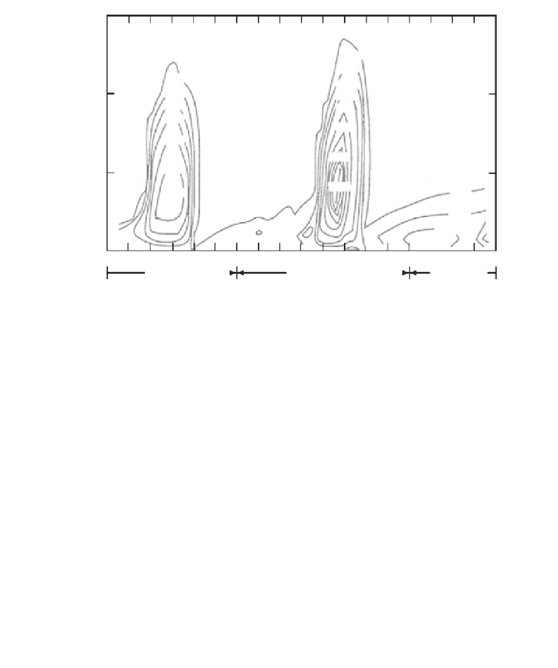
Figure 18.7
Measured TKE with height in daytime conditions at Wangara, Australia. (Redrawn from Yamada and Mellor,
1975, published with permission).
Figure 18.7 shows how TKE of air in the ABL is 'spun up' during the day and then
subsequently decays at night.
The turbulent kinetic energy in the ABL is present across a range of frequencies
and the shape of this spectrum evolves with time depending on local ambient
conditions. Figure 18.8a shows a typical spectrum for TKE in unstable conditions.
The terms in Equation (18.17) also have different spectra, and Fig. 18.8b shows the
spectra for the buoyant and shear production terms and the turbulent dissipation
term. This figure reveals that turbulence is largely produced at low frequency but
is mainly dissipated at high frequency. The energy present in large eddies provides
energy to smaller and smaller eddies until the secondary eddies so created are
small and the spatial gradients of variance in the viscous dissipation term,
, there-
fore large. The kinetic energy associated with motion in the turbulent air is then
dissipated through friction as heat.
e
Prognostic equations for variance of moisture and heat
The prognostic equation for the variance in the moisture content and heat
content of air in the ABL can be derived following procedures broadly analo-
gous to that used to derive Equation (18.13), the prognostic equations for the