Geoscience Reference
In-Depth Information
18
Observed ABL
Profiles: Higher
Order Moments
Introduction
The equations describing the evolution of the mean values of atmospheric variables
in the turbulent ABL were introduced in Chapter 17. It is appropriate next to
investigate how these equations control atmospheric behavior by considering
typical observed changes in mean variables and turbulent fluxes in the ABL during
the course of the day. For simplicity, it is helpful to do this while assuming the ABL
overlies a flat, horizontally homogeneous surface. This makes the equations
simpler to understand because it means terms that represent the rate of change of
mean values or turbulent fluxes with distance along the X and Y axes can be
assumed small in comparison with those that describe the rate of change along the
Z axis. If the terrain is flat, it is also plausible to assume that the mean wind speed
along the Z axis (i.e., subsidence) is zero.
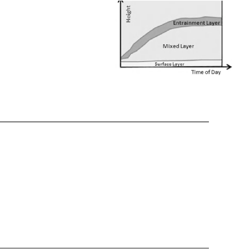
Nature and evolution of the ABL
In general terms, the lower atmosphere can be divided into the four main layers
which are diagnosed by the rate of change with height of virtual potential
temperature, wind speed, specific humidity and other scalar variables, as shown
in Fig. 18.1 for daytime conditions. The lowest layer, the
surface layer
, which has a
depth on the order of 100 meters, is strongly influenced by the aerodynamic
roughness of the underlying surface and by surface heating. In this layer, mean
atmospheric variables initially change rapidly with height but the rate of change
becomes progressively less away from the surface. During the day, air in the surface
layer is usually unstable because of surface warming but at night the surface layer
usually becomes stable as the surface cools by emitting longwave radiation.