Biomedical Engineering Reference
In-Depth Information
microscope. his is not a severe limitation. We are interested in the maximum aberration that we
would have to correct for in an adaptive optics system. It naturally occurs when focusing on the bot-
tom of the sample.
Note that in the case of the CFM, the aberrations are introduced in both the excitation and the emis-
sion paths. With the interferometer, we measure the aberrations of exactly this path, but because of the
single-pass nature the result of the measurement is lesser by a factor of two.
4.7 Data Acquisition
For the data shown in this chapter, we recorded 256 wavefronts corresponding to the 256 positions
within a 16 × 16 grid of focal positions within each specimen. A range of typical biological specimens
were chosen. he measurement spot of the interferometer travels across the ield of view, and for each
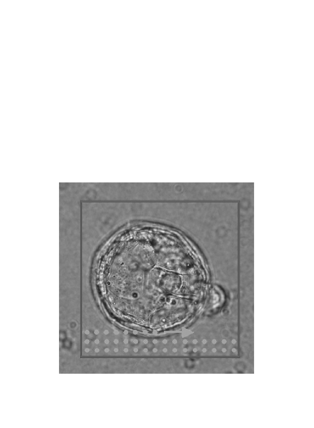
point a wavefront is recorded and the Zernike mode analysis is performed. To illustrate the scanning
process, a transmitted light image of a mouse blastocyst sample is shown in Figure 4.7. he green dots
correspond to positions for which a wavefront was recorded.
One scan takes less than ive minutes. he acquisition of the wavefront at each point involves the
recording of three interferogram images at relative phase steps of 0°, 120°, and 240°, which are then
processed to reconstruct the wavefront as discussed in
Section 4.8
.
he wavefront recorded for one particular position of the sample contains three contributions to
the total aberration, namely the static aberrations of the optical system, the static specimen-induced
Figure 4.7 (See color insert.)
Transmitted light image of the mouse blastocyst sample. he recording of
the wavefront at diferent raster positions is shown by the superimposed green dots. Two hundred and ity-six
wavefronts were recorded on a 16 × 16 grid. he size of the scan area indicated by the red frame is 130 × 130 μm.