Biomedical Engineering Reference
In-Depth Information
180
40000
40000
160
30000
30000
140
20000
20000
120
10000
10000
0
0
100
10
20
30
40
100
10
20
30
40
100
80
(a)
(b)
60
40000
40000
40
30000
30000
20
20000
20000
0
20
40
60
80
10000
10000
Depth (
μ
m)
0
0
10
20
30
40
100
10
20
30
40
100
(e)
(c)
(d)
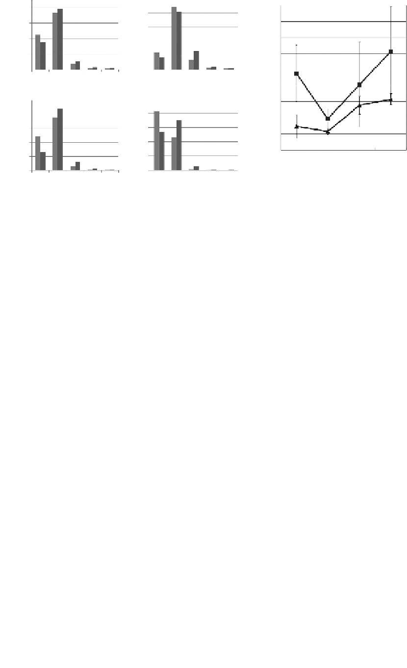
FIGuRE 16.11
Signal.improvement.ater.AO.compensation..(a-d).Histograms.for.the.number.of.pixels.accord-
ing.to.their.intensity;.the.
x
-axis.represents.the.intensity.of.pixels.the.same.as.in
.
Figure.16.9
,
.except.100.(100.means.
40%-100%.intensity.pixels.in.the.image)..he.
y
-axis.represents.the.number.of.pixels.in.the.intensity.range..he.let-
placed.columns.show.the.number.of.pixels.before.the.compensation,.and.the.right-placed.columns.show.the.result.
ater.compensation..Each.histogram.was.normalized.to.itself..he.distribution.at.(a).20.μm,.(b).40.μm,.(c) 60 μm,.
and.(d).80.μm.imaging.depth..(e).Percentage.improvement.according.to.imaging.depth..he.solid.line.with.triangles.
shows. the. improvement. with. background. rejection. (only. the. luorescent. area. was. calculated),. and. the. solid. line.
with.squares.shows.the.improvement.only.with.90-100%.intensity.pixels.
16.3.5 neuronal imaging in Mouse-Brain Slices Using Adaptive
optics-compensated two-Photon Microscopy
Both.muscle.tissues.have.high.scattering.coeicients.that.appear.to.be.the.major.limiting.factor.in.deep.
tissue.two-photon.imaging..It.is.of.interest.to.also.study.tissue.specimens.that.have.signiicantly.lower.
scattering,. and. therefore. allow. deeper. imaging.. For. this. purpose,. we. chose. mouse-brain. slices. with.
neurons. expressing. green. luorescent. protein. (GFP). driven. by. a. hy-1. promoter.. Adult. hy-1-GFP-S.
mice.were.perfused.transcardially.with.4%.paraformaldehyde.in.PBS..he.brains.were.removed,.and.
post-ixed. overnight. in. 4%. paraformaldehyde. and. sectioned. coronally. at. 200. μm. thickness. using. a.
vibratome..he.wavelength.of.the.excitation.light.was.890.nm,.and.a.40×.water-immersion.objective.
lens.(Achroplan.IR,.0.8.N;.Zeiss).was.used.with.a.number.11.2.coverslip..he.emission.signal.was.iltered.
with.a.green.ilter..he.ield.size.was.120.×.120.μm.over.256.×.256.pixels,.and.the.dwell.time.was.40.μs.
Figure.16.12.
shows.representative.mouse-brain.images.at.50.μm.depth.with.and.without.AO.compen-
sation..he.mouse-brain.specimen.contained.sparsely.distributed.GFP-expressing.neurons..he.image.
on.the.let.is.the.uncompensated.image,.and.the.image.on.the.right.is.the.compensated.image,.with.both.
processed.for.background.rejection..AO.compensation.was.performed.at.the.center.pixel,.and.scanning.
was.done.with.the.same.deformable.mirror.shape..he.compensated.image.showed.a.higher.signal.than.
the.uncompensated.one..To.compare.the.signal.level.of.two.images,.the.intensity.distributions.for.all.
pixels. are. shown. in.
Figure. 16.13
.
.
Figure. 16.13a
.
and
.
b.
show. histograms. for. the. intensity. distributions.
before. and. ater. compensation.. Since. the. structure. imaged. is. sparse,. the. histogram. is. dominated. by.
zero-intensity.pixels..Two.additional.igures.below.
Figure.16.13a
.and
.
b.
show.histogram.distributions,.
excluding.the.lowest.intensity.range..Again,.the.number.of.brighter.pixels.increased,.and.the.number.
of.darker.pixels.decreased,.ater.AO.compensation..For.the.improvement.trend.according.to.imaging.
depth,. mean. photon. counts. were. calculated. with. background. rejection.
.
Figure. 16.13c
. shows. the. per-
centage.improvement.from.the.mean.photon.counts.according.to.the.imaging.depth..We.see.a.general.