Biomedical Engineering Reference
In-Depth Information
9.4.1.2 Fresnel Approximation
Let us define (
x,y
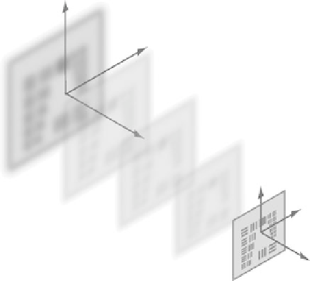
) and (ξ,η), respectively, as the lateral coordinates in the hologram plane (
z
= 0) and in
the reconstruction plane located at
z
=
d
, as illustrated in Figure 9.4. In the Fresnel approximation, it is
shown in Goodman (1968) that, given the wavefront ψ
0
(ξ,η) =
u
(ξ,η,
z
= 0)
I
(ξ,η,
z
= 0) in the hologram
plane, the reconstructed wave in an arbitrary plane
z
=
d
can be expressed as
(
)
exp
ikd
i d
i
π
λ
(9.4)
∫∫
ψ ξ η
( ,
)
=
ψ ξ η
( ,
)
exp
(
ξ
−
x
)
2
+
(
η
−
y
)
2
d
x y
,
d
0
λ
d
where λ is the wavelength. A review article by Schnars and Juptner specifically treats two of the possible
implementations of the above equation for numerical field propagation (Schnars and Juptner, 2002).
Here, let us summarize these two implementations.
9.4.1.3 convolution Approach to numerical Field Propagation
Equation 9.4 can be viewed as a convolution of the form
∞
∫
def
∫
(
f
⊗
g
)( ,
ξ η
)
=
f x y g
( , )
(
ξ
−
x
,
η
−
y
)
d d
x y
(9.5)
−∞
between
ψ
0
and a complex exponential kernel function of
x
and
y
. Using the equivalence between the
convolution in the space domain and the multiplication in the frequency domain, one can write ψ
d
as
exp
ikd
i d
(
)
π
λ
i
(
)
ψ
=
ψ
⊗
exp
x
2
+
y
2
d
0
λ
d
exp
ikd
i d
(
)
π
λ
i
(
)
{ }
⋅
=
F
−
1
F
ψ
F exp
x
2
+
y
2
0
λ
d
{
}
exp
ikd
i d
(
)
(
)
{ }
⋅
=
F
−
1
F
ψ
exp
i
πλ
d k
2
+
k
2
(9.6)
λ
0
x
y
where (F) and
(
F
−1
, respectively, denote the direct and inverse Fourier transform operator.
)
ψ
0
(
x
,
y
)
y
x
z
ψ
d
(
ξ
,
η
)
η
z
= 0,
Hologram plane
ξ
5
1
2
4
6
1
2
3
6
z
z
=
d
,
Image reconstruction plane
FIgurE 9.4
Hologram reconstruction. Convention for variables.