Biomedical Engineering Reference
In-Depth Information
The SHG emission directionalities between the tissues are significantly different and can be inter-
preted by the difference in fibril assembly. Using a space-filling analysis of TEM images, we found the
packing of the fibrils in the malignant tissue to be more regular relative to the normal (10% vs. 15%
interfibrillar space, respectively). Based on our mathematical model of SHG in fibrillar tissues [23], the
fibril assembly of the malignant tissue, that is, regularly packed fibrils on the order of the coherence
length, would give rise to efficient backward emitted SHG [23]. In contrast, the more random assembly
in the normal would result in more predominantly forward initial emission directionality (i.e., higher
%
F
SHG
), as was extracted from the simulation of the data.
6.4.2.2 SHG Attenuation Measurements and Simulations
The averaged normalized forward attenuation data with standard errors are shown in Figure 6.12a for
the normal (
n
= 5) and malignant (
n
= 3) tissues. Unlike the
F/B
response, the SHG attenuation provides
no clear separation between the tissues. To understand this effect, we need to consider all the factors that
give rise to the measured attenuation. As described earlier, it is not possible to directly determine rela-
tive χ
(2)
values in intact tissues as the measured signal is convolved with scattering when the tissues are
thicker than one MFP or ~50 microns. However, this can be achieved using much thinner H&E histo-
logical sections (~5 microns). We note that the eosin staining does not contribute to the observed SHG.
Measurement of the relative SHG intensities from these sections yields a factor of 3.9 ± 0.1 (
p
< 0.005)
increased brightness for the cancer.
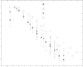
We now use all our measured factors as inputs into Monte Carlo simulations of the SHG attenuation.
The simulated data for the normal (open squares) and malignant tumors (open circles) based on the
bulk optical parameters (see Table 6.2) and the relative χ
(2)
values are shown in Figure 6.12b. Like the
experimental data, the simulations are highly similar for these two tissues. However, the rate of decay
of the simulated SHG intensity is somewhat greater for the experimental data, where the differences are
most pronounced at the bottom of the slice. While an exact match was not obtained, this approach still
allows us to understand the similarity in the measured data for these tissues. It arises from the offsetting
parameters of the increased conversion efficiency (χ
(2)
) and larger μ
s
for the cancers, as these separately
would result in slower and faster normalized attenuations, respectively.
(a)
(b)
1.0
Normal experimental
Normal
1.0
Normal simulated
Cancer
Cancer experimental
0.8
Cancer simulated
0.8
0.6
0.6
0.4
0.4
0.2
0.2
0
20
40
60
80
100
0
20
40
60
80
100
120
Depth (microns)
Depth (microns)
FIgurE 6.12
Forward SHG attenuation data and simulations for normal and malignant ovarian biopsies.
(a) Shows the experimental data for normal (squares) and cancer (circles). (b) Shows the experimental data (closed
circles and squares) every 10 microns and the simulations (open circles and squares) based on the measured bulk
optical parameters in Table 6.1 and the relative χ
(2)
values that were determined from the histological sections.
(Reproduced from Nadiarnykh, O. et al. 2010.
BMC Cancer
10:94.)