Biomedical Engineering Reference
In-Depth Information
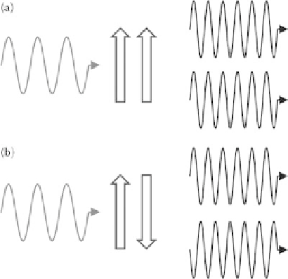
FIgurE 5.2
Dipole orientation and coherent summation. The figure shows examples of the HRS waves produced
by two pairs of irradiated dipoles. The HRS wave generated by each dipole is represented on the right. (a) If the
molecules are parallel, their HRS waves are in phase with the driving field and can interfere constructively. (b) If
the molecules are antiparallel, their HRS waves have opposite phases and interfere destructively. (Inspired from
Mertz, J. P.S.B.R. Masters, ed. Applications of second-harmonic generation microsocpy. In
Handbook of Biomedical
Nonlinear Optical Microscopy
, 2008. Oxford: Oxford University Press. By permission of Oxford University Press.)
is clear that, considering a population of N molecules, the resulting signal is not simply the sum of the scat-
tered powers from each molecule but rather the result of their overall interference, which is determined by
the orientation distribution within the population. Therefore, the resulting HRS power strongly depends
on the angular distribution of the population. In the extreme case of randomly oriented molecules, the
HRS contributions have random phases, and the total HRS signal, produced incoherently, will scale as the
number of radiating molecules N. On the other hand, if the molecules are well aligned, the phases of the
individual HRS contributions are locked to the phase of the driving field. The coherent production of HRS
occurring in the latter case is called second-harmonic generation (SHG) and its total power scales as
N
2
. A
quantitative description of these processes is provided in the following section.
The dependence of signal on isotropic versus anisotropic HRS emitters distributions is the basis for
high-contrast imaging of ordered structures. Moreover, the anisotropic distribution of the scatterers is
reflected in coherent summation producing a polarized SHG signal. Quantitative measurements of SHG
polarization anisotropy can, therefore, provide information on the scatterers distribution itself.
5.3 SHG Polarization Anisotropy
The general description of the polarization
P
in a medium is given by
P
=
χ
( )
1
E
+
χ
( )
2
EE
+
(5.2)
This equation is the bulk equivalent of Equation 5.1. The second-order susceptibility χ
(2)
describes
the relation between all the components of the polarization and the electric-field vectors for sum and
difference frequencies generation. In the general case of three-wave mixing, the susceptibility tensor
χ ω ω
ijk
( )
(
2
1 2
is a third-rank tensor and contains 27 (3 × 3 × 3) elements. In the specific case of SHG, in
which two fields with the same frequency (ω
1
= ω
2
= ω) generate a third field with frequency 2ω, each
component of the second-order polarization can be expressed as
,
)