Biomedical Engineering Reference
In-Depth Information
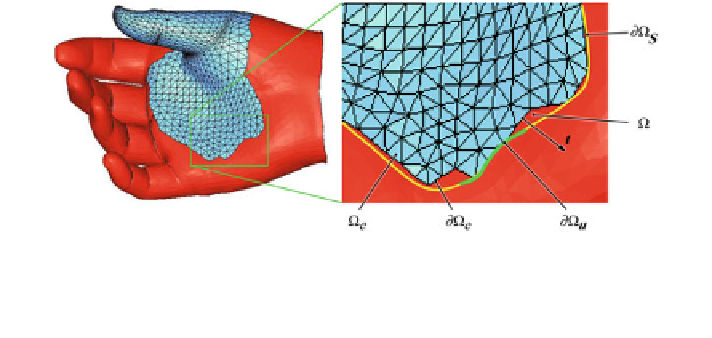
Fig. 3.26 Discretized (meshed) problem domain X with domain boundary oX
¼
oX
u
þ
oX
S
where oX
u
and oX
S
are the Dirichlet and von Neumann boundary conditions, respectively. X
e
and oX
e
denote element domain and element boundary, respectively; t is the surface traction
vector
The problem solution is explicitly determined in terms of discrete values of
some field variables, e.g. displacements in structural mechanics, at the element
nodes. Unknown variation of field variables at non-nodal points are approximated
across the element domain by interpolating the field variable values at the element
nodes using element shape functions (also referred to as interpolation functions).
This method is referred to as element interpolation.
The element shape functions, most often polynomial forms of the field vari-
ables, are predetermined, known functions which thus describe the continuous
variation of the field variable within each finite element.
With the terms previously introduced, the error sources of a FEM solution, as
illustrated in Fig.
3.25
, can be described in more detail. While solution errors occur
as a result of the calculation procedure and include truncation and round off errors,
discretization errors refer to errors based on distorted elements due to complex
geometries or boundary representation. Modeling errors result from the fact that
finite elements might not precisely describe the behavior of the physical problem.
The general approach to the finite element method is summarized as follows:
1. Discretization of the problem domain into a set of finite elements.
2. Description of the mechanical behavior of each finite element involving
restatement of the strong form of the boundary value problem in its integral
or weak form (alternatively to the theorem of minimum potential energy)--
(in stress analysis, the weak form can alternatively be developed from the
principle of virtual work).
3. Derivation of finite element interpolation functions.
4. Development of the finite element equations using the weak form, employing
Galerkin's method.
5. Assembly of the finite element equations to obtain the global system of
equations.
6. Imposition
of
the
boundary
conditions
and
solution
of
the
assembled
equations.