A Model of Electromechanical Coupling in the Small Intestine - Multiscale Computer Modeling in Biomechanics and Biomedical Engineering - page 187

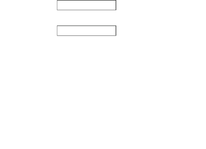
Anatomical model

Electrical model

Mechanical Model [Ca ]

2+

i

Passive model Active model

Total Tension

Deformation Intraluminal pressure

Fig. 4 Schematic of the electromechanical coupling process used in this simulation. At each
solution step, the electrical component is solved first, and the relevant variables in the cell
models, i.e., [Ca 2 þ ] i , is linked to the active component of the mechanical model. The active
component is solved together with the passive component to update the deformation of the
geometric model

The electrical model was solved for ½ Ca 2 þ i values (Fig. 3 ), which are then fed to
the active mechanics component. Resultant active tension was incorporated into the
finite deformation equations that, together with the passive constitutive law,
specified deformation of the geometry. The mesh was updated with this new
geometry before the next solution step. Stress and radial measurements along the
small intestine were used to approximate the intraluminal pressures at various axial
locations along the anatomical model.

4.1 Finite Deformation Theory

In the small intestine, peristalsis can occlude more than 70 % of the diameter of
the lumen [ 1 ]. Such large and nonlinear deformation presents a challenge to the
conventional linear and small-strain deformation theory. In this case, a more
fundamental approach of finite elasticity is needed when using the mechanical
behavior of elastic materials which undergo large strains. Stress is another
important measure in mechanical deformation, and it can also vary greatly
between the undeformed and deformed states as the smooth muscle fiber elongates
under large strains.
Formulation of finite elasticity is a relatively more complex procedure than
linear elasticity formulations, as it involves ''tracking'' the deforming material. In