A Model of Electromechanical Coupling in the Small Intestine - Multiscale Computer Modeling in Biomechanics and Biomedical Engineering - page 185

0.0 s 0.5 s 1.0 s

1.5 s 2.0 s 2.5 s

3.0 s 3.5 s 4.0 s

4.5 s 5.0 s 5.5 s

6.0 s 6.5 s 7.0 s

7.5 s 8.0 s

-7 0 -30

V m (mV)

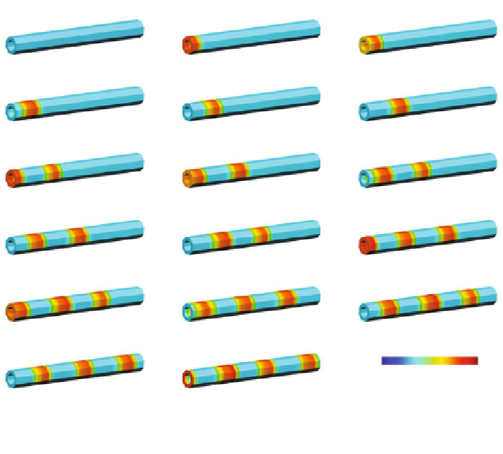
Fig. 3 Simulated intestinal electrical activity. Visualization of slow wave membrane potential at
regular intervals in an idealized intestinal model, from 0 to 8 s. The color bar indicates
membrane potential values in mV, ranging from 70 (blue)to 30 mV (red)

ot ¼ V t þ 1

o V m V t m

Dt

m

ð 12 Þ

The discretized bidomain equations can be solved sequentially, with the V m term
from Eq. ( 11 ) is used to update Eq. ( 10 ) at each time step.
In our simulation, as an example of intestinal slow wave propagation, the
smooth muscle cell model was solved at tissue-level using the bidomain formu-
lation implemented within a grid-based (solution points) finite element framework.
Four grid points were assigned in each n-direction of the segment model in
Fig. 1 b, to make a total of 64 grid points per element, and 8,192 in the whole
geometry. The intestinal slow wave propagation was simulated for 2.8 s and
visualized over the intestinal geometry (Fig. 3 ). Boundary conditions of zero
current flux through the cell membrane boundary condition were assigned to the
model. Anisotropic tissue conductivities assigned to the fiber, sheet and sheet-
normal directions were 1, 0.5 and 0.019 mS mm 1 respectively in the intracellular
domain and 1, 0.5 and 0.236 mS mm 1 in the extracellular domain.
The frequency of the simulated intestinal slow wave activity was 23 cpm, with
a propagating velocity of 5 mm s 1 . In this initial simulation, the slow wave