Biomedical Engineering Reference
In-Depth Information
d
T
P
X
T
P
T
P
XL
XL
T
P
T
P
XL
XL
XL
ï
ï
T
P
PVHF
LFP
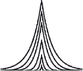
Figure 4.5:
Time and space solution in a passive cable.
the left panel, action potentials shown at
x
2
cm
(red). Notice that although the
action potential shape does not change, there is a delay in timing of the upstroke. The right panel shows
a snapshot of the voltage along the cable at
t
=
1
cm
(black) and
x
=
40
msec
. Notice that the when propagation is from left to
right, the spatial plot has the shape of a reversed action potential.To understand why, consider the location
at
x
=
2
cm
. In the right panel, at 40
msec
, the point is at rest. The shape in the left panel, however, is
moving the right so eventually the sharp spike will reach
x
=
=
2
cm
. From the right panel we know that
=
this occurs at approximately
t
55
msec
. In space, the reversed action potential shape will continue to
move the right causing the location at
x
=
2
cm
to undergo all of the phases of an action potential.
ï
ï
ï
ï
ï
ï
ï
ï
7LPHPVHF
6SDFHFP
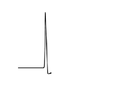
Figure 4.6:
Propagation down an active cable.
For uniform propagation down a cable and uniform
I
ion
everywhere in the cable, we say that
V
m
(x, t)
=
V
m
(x
−
θ(t)
(4.26)