Biomedical Engineering Reference
In-Depth Information
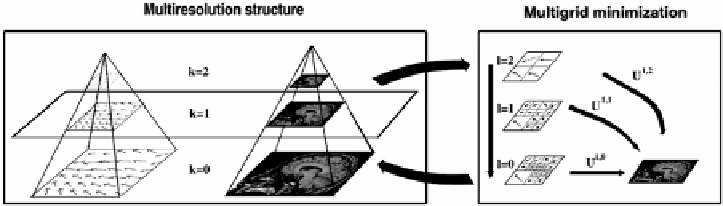
Figure 8.2:
Example of multiresolution/multigrid minimization. For each res-
olution level (on the left), a multigrid strategy (on the right) is performed. For
legibility reasons, the figure is a 2D illustration of a 3D algorithm with volumetric
data.
convergence rate as compared to the standard iterative solvers (such as Gauss-
Seidel).
At grid level
,
={
n
,
n
=
1
,...,
N
}
is the partition of the volume
B
into
N
cubes
n
. At each grid level
corresponds a deformation increment
T
k
,
that is defined as follows: A 12-dimensional parametric increment deformation
field is estimated on each cube
n
, hence the total increment deformation field
d
w
k
,
is piecewise affine. At the beginning of each grid level, we construct a
reconstructed volume with the target volume
f
k
(
s
,
t
2
) and the field estimated
previously (see section 8.3.2). We compute the spatial and temporal gradients at
the beginning of each grid level and the increment deformation field
d
w
k
,
is ini-
tialized to zero. The final deformation field is hence the sum of all the increments
estimated at each grid level, thus expressing the hierarchical decomposition of
the field.
Contrary to block-matching algorithms, we model the interaction between
the cubes (see Section 8.3.2) of the partition, so that there is no “block-effects”
in the estimation. At each resolution level
k
, we perform the registration from
grid level
c
until grid level
f
. Depending on the application, it may be useless
to compute the estimation until the finest grid level, i.e.,
f
=
0. We will evaluate
this fact later on (see section 8.3.3).
Adaptive Partition.
To initialize the partition at the coarsest grid level
c
,
we consider a segmentation of the brain obtained by morphological operators.
After a threshold and an erosion of the initial volume, a region growing pro-
cess is performed from a starting point that is manually chosen. A dilatation