Structure Contouring - 3-D Structural Geology - page 76

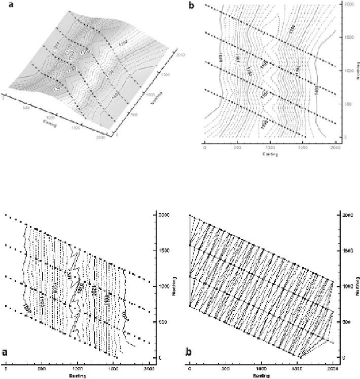
Fig. 3.15. Map made by inverse-distance interpolation (weighting exponent 3.5) of points along cross sections
from data in Fig. 3.14. Lines of black squares are control points. a Oblique view. b Structure contour map
Fig. 3.16. Map made by triangulation of points along cross sections from data in Fig. 3.14. Lines of
black squares are control points. a Structure contour map. b TIN network
structural trend. Nearest neighbors are the closest points on adjacent traverses. This
problem can be overcome by orienting traverses parallel and/or perpendicular to the
structural trend, or by mapping based on the structural trend (Sect. 5.5).
Non-cylindrical folds pose a greater challenge for accurate mapping. The fold in
Fig. 3.17a is a simple flat-topped anticline with limbs that converge to the south and
disappear, giving a conical geometry. Sampled along three traverses perpendicular to
the average crestal trend, the reconstruction does only a fair job of reproducing the
original geometry. The fold limbs are reproduced but the flat crest and the plunging
nose are misrepresented. Mapping based on 3-D dip domain interpretation (Sect. 6.7)
is the most accurate approach for this style of structure.