Geology Reference
In-Depth Information
9.4
Analysis of Uniform Dip
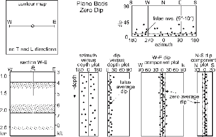
The dip component diagrams are the primary noise reduction strategy in SCAT analy-
sis. For zero dip the azimuth of the dip is random (actually stratigraphic scatter) and
the dip amount shows a false positive average (Fig. 9.8). As the amount of homoclinal
dip increases (Figs. 9.9, 9.10) the concentration of points becomes sharper. The com-
ponent plots for zero dip show the correct zero average (Fig. 9.8). Low and moderate
planar dips (Figs. 9.9, 9.10) show their true dip values on the transverse component plots
because these are in the dip direction. The longitudinal dip components average zero
because they are in the strike direction. The zero
L
component average (Figs. 9.9, 9.10)
confirms the choice of the
L
and
T
directions.
9.5
Analysis of Folds
Folds produce distinctive curves on the dip vs. depth plots. The azimuth vs. depth plot
shows the reversal of azimuth at the crest of the fold, CP (Figs. 9.11-9.13). The dip com-
ponent plots are the most informative. The transverse component plots all cross the zero
dip line at the crest of the anticline (CP), show an inflection point at the axial plane (AP)
and show a dip maximum at the inflection plane (IP) that separates anticlinal curvature
from synclinal curvature. Any variations in plunge are apparent on the longitudinal com-
ponent plot. The non-plunging fold (Fig. 9.11) is defined by a straight line on the plot of
Fig. 9.8.
Model map, cross section and SCAT plots for zero dip. (After Bengtson 1981a)