Biomedical Engineering Reference
In-Depth Information
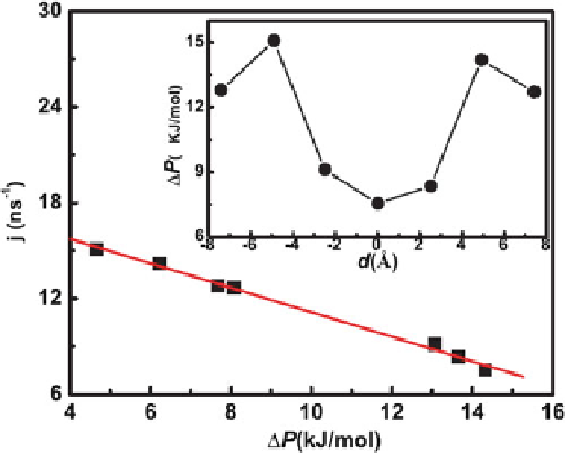
Fig. 1.28
The water flux
j
for different P and (inset) P for different
d
. In this figure, P
is the difference between the maximum and the minimum of the interaction potential, which is
usually used to characterize the potential profiles (reprinted from [
131
]. Copyright 2011 American
Physical Society)
From Fig.
1.28
, we can find the M-type profile of P , showing that P
approaches to the minimum as the narrow portion moves to the middle of the SWNT.
The corresponding value of P is
7.7 kJ mol
1
, only half of the P for
d
D
4.9
or 4.9 A. Consequently, the flux for
d
D
0 A approaches to the maximum. From the
simulation results shown in Fig.
1.28
, we can find that the water flux decreases
almost linearly with increasing P . The data can be well fitted by the following
formula:
j
D
j
0
.1
P ="/;
where "
18.1 kJ mol
1
and
j
0
D
21.7 ns
1
. According to the above fitted formula,
the net water flux would decrease to zero when P
D
"
18:1kJ mol
1
.To
check the validity of the prediction, a system of depth
D
2.3
˚
Aand
d
D
4.9 A
was simulated, and then the simulation result shows that the net water flux is still
0.6 ns
1
and the matching P is
22 kJ mol
1
, implying that the fitted linear
law is a good fit only for P < 16kJmol
1
.
From the above simulation results and discussions, it is concluded that the water
flux is not only sensitive to the strength of the deformation but also significantly
influenced by the location of the deformation. When the deformation is just located
in the middle of the nanotube, forming an hourglass-shaped region, the water flux
across the nanotube reaches a maximum. Simulation results furthermore indicate
that the hourglass shape is more convenient for water molecules to pass through the
nanotube than a funnel shape.