Biology Reference
In-Depth Information
Time domain—Time-correlated single-photon counting
S
2
S
1
S
2
Fluorescence
lifetime
D
t
2
D
t
2
D
t
1
S
0
S
0
S
0
D
t
1
D
t
2
D
t
n
D
t
2
D
t
1
D
t
n
Laser pulse
Emitted photon
Previously emitted photon
Fit curve
Frequency domain—Phase and modulation lifetime
Modulated excitation
Fluorescence emission
Fitting for each pixel
Phase lifetime (
t
j
)
4ns
j
1
j
2
Phase shift (
j
)
Modulation lifetime (
t
m
)
reference
Elapsed time
1ns
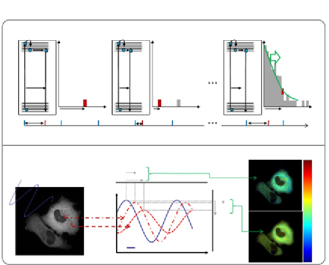
Figure 5.13 Principle of lifetime measurements. (A) In the time domain, a pulsed laser is
used to excite fluorophores. The time between photon excitation and emission is mea-
sured and accumulated to get an histogram of photon emission time. Fluorescence life-
time is then estimated from the slope of this exponential decay. (B) In the frequency
domain, a modulated excitation is used to excite the sample. Monitoring of the fluores-
cence phase and modulation shift compared to a reference with known fluorescence
lifetime is used to calculate phase and modulation lifetimes.
for TCSPC experiments, which, however, necessitates particular atten-
tion during photon decay curves analysis;
a photon counting card. All the systems rely on the same principle,
which is based on a time amplitude converter. It consists in a linear volt-
age ramp started by the arrival of a photon and stopped by the next laser
pulse. The output voltage will thus be proportional to the photon arrival
time. However, the ramp is triggered only by a photon arrival followed
by a laser pulse, which means that if two photons are acquired between
two laser pulses, only the first photon will be measured. This is the “pulse
pile-up” effect (
Fig. 5.14A
). To avoid this statistic selection of fastest
photons, one has to limit the acquisition frequency to one-hundredth
of the excitation frequency (giving rise to an error every 10,000 pho-
tons), which explains the longer acquisition time of this technique.
An example of such a setup
23
is presented in
Fig. 5.14B
.
Search WWH ::

Custom Search