Graphs and paths - Data Structures and Problem Solving Using Java - page 543

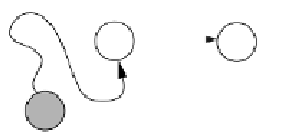
Figure 14.20 illustrates a fundamental principle: If a path to vertex v has
cost D v and w is adjacent to v , then there exists a path to w of cost D w = D v + 1.
All the shortest-path algorithms work by starting with D w =

∞

and reducing its
value when an appropriate v is scanned. To do this task efficiently, we must scan
vertices v systematically. When a given v is scanned, we update the vertices w
adjacent to v by scanning through v 's adjacency list.

From the preceding discussion, we conclude that an algorithm for solving
the unweighted shortest-path problem is as follows. Let D i be the length of the
shortest path from S to i . We know that D S = 0 and that D i =

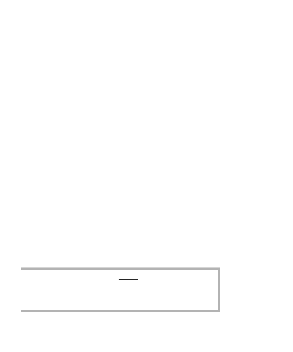
The roving eyeball
moves from vertex
to vertex and
updates distances
for adjacent verti-
ces.

∞

initially for all

i S . We maintain a roving eyeball that hops from vertex to vertex and is ini-

tially at S . If v is the vertex that the eyeball is currently on, then, for all w that
are adjacent to v , we set D w = D v + 1 if D w =

≠

∞

. This reflects the fact that we
can get to w by following a path to v and extending the path by the edge
( v , w )—again, illustrated in Figure 14.20. So we update vertices w as they are
seen from the vantage point of the eyeball. Because the eyeball processes each
vertex in order of its distance from the starting vertex and the edge adds
exactly 1 to the length of the path to w , we are guaranteed that the first time
D w is lowered from

∞

, it is lowered to the value of the length of the shortest
path to w . These actions also tell us that the next-to-last vertex on the path to w
is v , so one extra line of code allows us to store the actual path.
After we have processed all of v 's adjacent vertices, we move the eyeball
to another vertex u (that has not been visited by the eyeball) such that
. If that is not possible, we move to a u that satisfies . If
that is not possible, we are done. Figure 14.21 shows how the eyeball visits
vertices and updates distances. The lightly shaded node at each stage repre-
sents the position of the eyeball. In this picture and those that follow, the
stages are shown top to bottom, left to right.

D u D v ≡ D u = D v + 1

The remaining detail is the data structure, and there are two basic actions
to take. First, we repeatedly have to find the vertex at which to place the eye-
ball. Second, we need to check all w 's adjacent to v (the current vertex)
throughout the algorithm. The second action is easily implemented by iterat-
ing through v 's adjacency list. Indeed, as each edge is processed only once,

All vertices adja-
cent to v are found
by scanning v 's
adjacency list.

figure 14.20
If w is adjacent to v
and there is a path to
v , there also is a path
to w.

D v +1

D v

v w

0

S