Java Reference
In-Depth Information
12.1.2
huffman's algorithm
How is the coding tree constructed? The coding system algorithm was given
by Huffman in 1952. Commonly called
Huffman's algorithm,
it constructs an
optimal prefix code by repeatedly merging trees until the final tree is obtained.
Throughout this section, the number of characters is
C
. In Huffman's
algorithm we maintain a forest of trees. The
weight
of a tree is the sum of the
frequencies of its leaves. times, two trees, and , of smallest
weight are selected, breaking ties arbitrarily, and a new tree is formed with
subtrees and . At the beginning of the algorithm, there are
C
single-
node trees (one for each character). At the end of the algorithm, there is one
tree, giving an optimal Huffman tree. In Exercise 12.4 you are asked to prove
Huffman's algorithm gives an optimal tree.
Huffman's algorithm
constructs an opti-
mal prefix code. It
works by repeat-
edly merging the
two minimum-
weight trees.
C
-
1
T
1
T
2
T
1
T
2
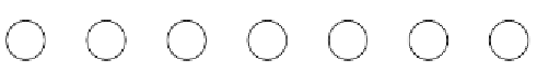
An example helps make operation of the algorithm clear. Figure 12.6
shows the initial forest; the weight of each tree is shown in small type at the
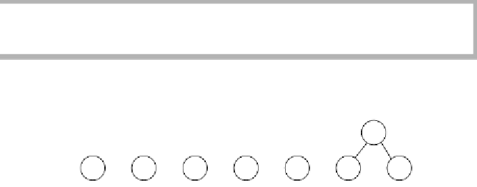
root. The two trees of lowest weight are merged, creating the forest shown in
Figure 12.7. The new root is
T
1. We made
s
the left child arbitrarily; any tie-
breaking procedure can be used. The total weight of the new tree is just the
sum of the weights of the old trees and can thus be easily computed.
Now there are six trees, and we again select the two trees of smallest
weight,
T
1 and
t.
They are merged into a new tree with root
T
2 and weight 8,
as shown in Figure 12.8. The third step merges
T
2 and
a,
creating
T
3, with
weight . Figure 12.9 shows the result of this operation.
After completion of the third merge, the two trees of lowest weight are the
single-node trees representing
i
and
sp.
Figure 12.10 shows how these trees
are merged into the new tree with root
T
4. The fifth step is to merge the trees
with roots
e
and
T
3 because these trees have the two smallest weights, giving
the result shown in Figure 12.11.
Finally, an optimal tree, shown previously in Figure 12.4, is obtained by merg-
ing the two remaining trees. Figure 12.12 shows the optimal tree, with root
T
6.
Ties are broken
arbitrarily.
10
+
8
=
18
figure 12.6
Initial stage of
Huffman's algorithm
10
15
12
3
4
13
1
a
s
t
e
i
sp
nl
figure 12.7
Huffman's algorithm
after the first merge
4
T
1
10
15
12
4
13
t
a
e
i
sp
s
nl


Search WWH ::

Custom Search