Algorithm analysis - Data Structures and Problem Solving Using Java - page 189

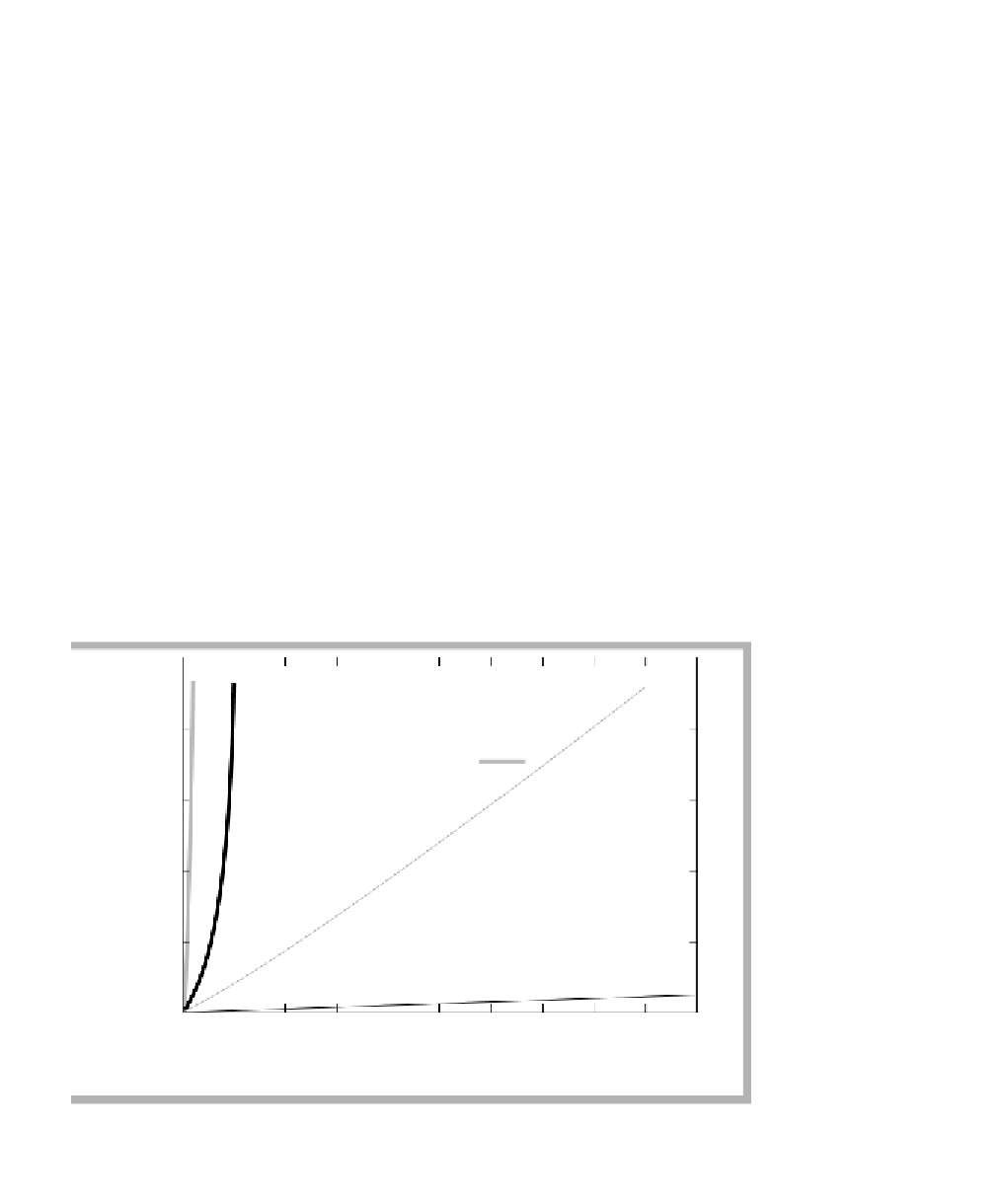
items, and the running times range from 0 to 10 microseconds. A quick glance
at Figure 5.1 and its companion, Figure 5.2, suggests that the linear, O( N log N ),
quadratic, and cubic curves represent running times in order of decreasing
preference.

An example is the problem of downloading a file over the Internet. Suppose
there is an initial 2-sec delay (to set up a connection), after which the download
proceeds at 160 K/sec. Then if the file is N kilobytes, the time to download is
described by the formula . This is a linear function .
Downloading an 8,000K file takes approximately 52 sec, whereas download-
ing a file twice as large (16,000K) takes about 102 sec, or roughly twice as
long. This property, in which time essentially is directly proportional to amount
of input, is the signature of a linear algorithm , which is the most efficient algo-
rithm. In contrast, as these first two graphs show, some of the nonlinear algo-
rithms lead to large running times. For instance, the linear algorithm is much
more efficient than the cubic algorithm.
In this chapter we address several important questions:

Of the common
functions encoun-
tered in algorithm
analysis, linear rep-
resents the most
efficient algorithm.

TN () = N ⁄ 160 + 2

Is it always important to be on the most efficient curve?

n

How much better is one curve than another?

n

How do you decide which curve a particular algorithm lies on?

n

How do you design algorithms that avoid being on less-efficient
curves?

n

figure 5.2
Running times for
moderate inputs

1

Linear
O( N log N )
Quadratic
Cubic

0.8

0.6

0.4

0.2

0

0 1000 2000 3000 4000 5000 6000 7000 8000 9000 10000

Input Size ( N )