Geology Reference
In-Depth Information
Field at the lower sensor
Field at the upper sensor
“Gradient”
Metres
20
0
Source A
5
Source B
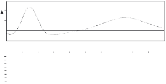
Figure 3.5
Inverse-cube law effects in magnetic gradiometry. The dotted
curve shows the magnetic effects of the two bodies as measured at the ground
surface, and the dashed curve shows the effects 1 metre above the surface.
The solid curve shows the differential effect. In the case of Source A, the
difference ('gradient') anomaly has 80% of the amplitude of the anomaly
measured at ground level. In the case of the deeper (but also stronger)
Source B, the total field anomaly amplitudes at the two sensors are much
more similar and the difference anomaly is therefore small.
Use of two sensors minimises thermal drift effects, reduces the effect
of errors in orientation, emphasises local sources and virtually eliminates
the effects of diurnal variations, including micropulsations. It is, however,
necessary to ensure that the two are very precisely aligned and are in ther-
mal equilibrium with each other and the environment. Three-component
fluxgates can eliminate the need for precise orientation or, alternatively, can
provide information on field direction as well as field strength.
3.4 Magnetic Surveys
Although absolute numerical readings are obtained (and can be repeated) at
a keystroke with proton and caesium magnetometers, faulty magnetic maps
can still be produced if simple precautions are ignored. For example, all
base locations, whether used for repeat readings or for continuous diurnal
monitoring, should be checked for field gradients. A point should not be used
as a base if moving the sensor by a metre produces a significant change.
3.4.1 Starting a survey
The first stage in any magnetic survey is to check the magnetometers (and
the operators). Operators can be potent sources of magnetic noise, although
the problems are much less acute when sensors are on long poles than
when they are carried in backpacks or when, as with fluxgates, they must be