GRAVITY METHOD - Field Geophysics - page 60

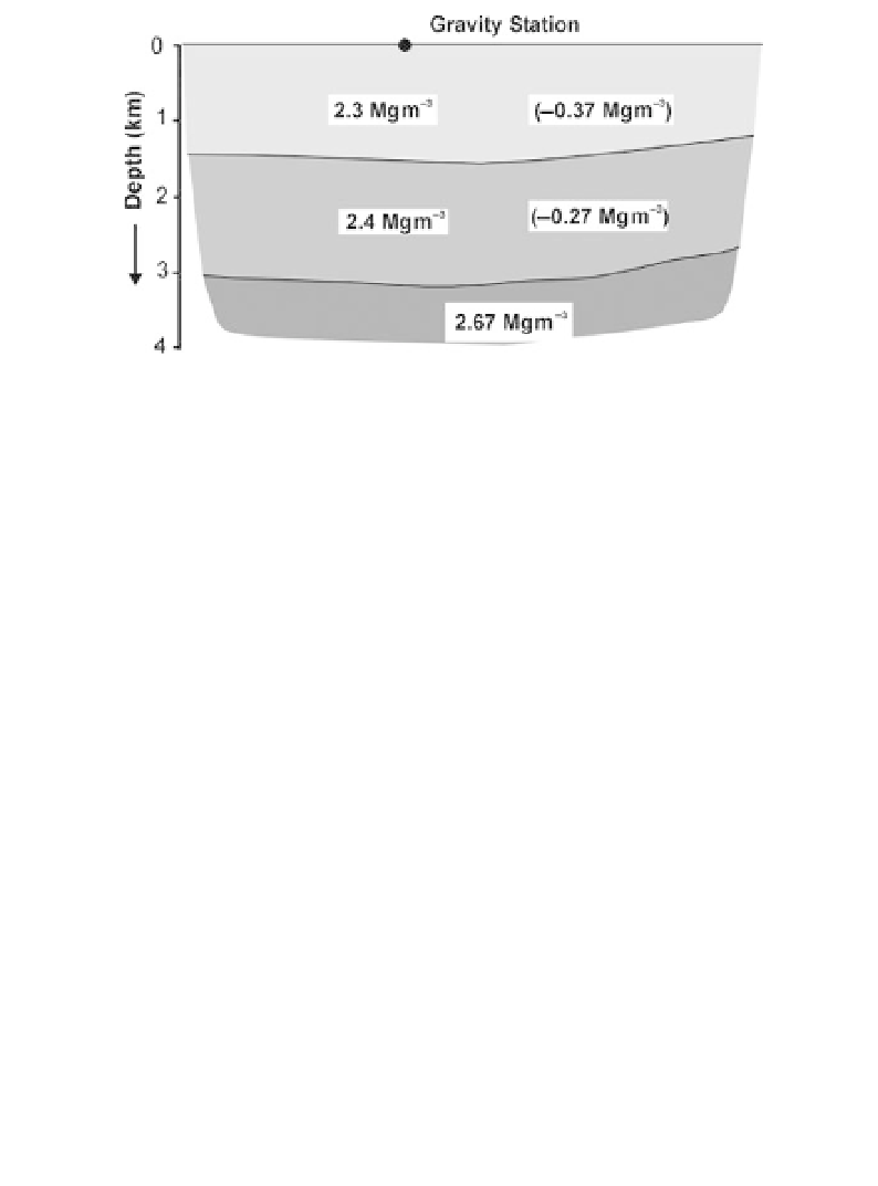
Figure 2.11 Sedimentary basin model suitable for Bouguer plate methods
of approximate interpretation. Modelling is usually done in terms of density
contrasts with basement, here assigned the standard 2.67 Mg m − 3 crustal

density. (See Example 2.1).

be needed for each station in rugged areas. Additional notebook columns
may be reserved for tidal and drift corrections, since drift should be cal-
culated each day, but these calculations are now usually made within the
meters themselves, or on laptop PCs or programmable calculators, and not
manually in field notebooks.
Each loop should be annotated with the observer's name or initials, the
meter serial number and calibration factor, and the base station number
and gravity value. It is also useful to record the difference between local
and 'Universal' time (GMT) on each sheet, as a reminder for when tidal
corrections are being calculated.
Gravity data are expensive to acquire and deserve to be treated with
respect. The general rules of Section 1.5.2 should be scrupulously observed.

Example 2.1
In Figure 2.11, if the standard crustal density is taken to be 2.67 Mg m − 3 ,
the effect of the upper sediment layer, 1.5 km thick, would be approximately
1.5 × 0.37 × 40 = 22 mGal at the centre of the basin.
The effect of the deeper sediments, 1.6 km thick, would be approximately
1.6 × 0.27 × 40 = 17 mGal.
The total (negative) anomaly would thus be about 39 mGal.