Geoscience Reference
In-Depth Information
For extreme cases of “unusual” distributions of residuals, a technique called “normal quan-
tile transform” (NQT) can be used to ensure that the transformed residuals have a Gaussian
distribution (see, for example, the work of Kelly and Krzysztofowicz (1997); Montanari and
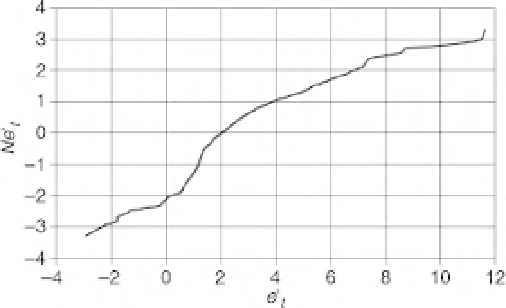
Brath (2004); Gotzinger and Bardossy, 2008). This is achieved by taking a time series of resid-
uals and ranking them from high to low. The quantiles of the resulting cumulative distribution
are then taken as the quantiles of a standard Gaussian distribution (see Figure B7.1.1). Gaussian
likelihood theory can then be applied to the transformed values (though again the series of
transformed residuals might still be correlated). Personally, I find this shoehorning of complex
residuals that might have non-stationary statistics into Gaussian form somewhat disturbing. It
is true that it allows the power of the statistical theory to be applied but in a way that might
have the effect of overstimating the information content of the residuals (including the extreme
stretching of the likelihood surface noted above) and therefore lead to overconditioning. Other
forms of transformation are also possible. Montanari and Toth (2007), for example, use a spec-
tral domain decomposition of the residuals leading to a likelihood function derived by Whittle;
while Schaefli and Zehe (2009) use a wavelet decomposition of the residuals.
Figure B7.1.1
A normal quantile transformplot of the distribution of the actual model residuals (horizontal
axis) against the standardised scores for the normal or Gaussian distribution (vertical axis) (after Montanari
and Brath, 2004, with kind permission of the American Geophysical Union).
There are two important points to remember about likelihood functions of this type. The
first is that they are based on treating the residual errors as only varying statistically or in
an aleatory way. The second is that the assumptions about the structure should always be
checked against the actual series of residuals for a model run. This is only usually done for
the maximum likelihood model found (which does not necessarily imply that the same error
structure applies throughout the parameter space). Engeland
et al.
(2005) show an example
of good practice in this respect; Feyen
et al.
(2007) do not. The latter used an assumption of
independent and uncorrelated errors in the identification of the maximum likelihood model
but then showed that the residuals were highly correlated in time. They did not go back and
repeat the analysis using a likelihood function that included autocorrelation. This means that
the resulting posterior parameter distributions are biased.
There is actually a further point that should be recalled here. The proportionality of Equation
(B7.1.3) derives from the work of Gauss in the early 19th century. It is the basis for all the widely
used statistical theory based on squared errors. It is, however, a choice. At much the same time,
Laplace proposed an alternative error norm based on a proportionality to the absolute error
(see Tarantola, 2006). Before the days of digital computers, this was much less analytically
tractable than the Gauss assumption, so did not attract so much attention. There are arguments