Geoscience Reference
In-Depth Information
x
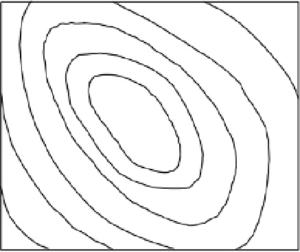
Parameter 2
Figure 7.1
Response surface for two parameter dimensions with goodness of fit represented as contours.
of parameter values. The ranges of the parameters define the parameter space. Plotting the resulting
values of goodness of fit defines a parameter
response surface
, such as that shown as contours in
Figure 7.1 (see also the three-dimensional representation in Figure 1.7). In this example, 10 discrete
increments would require 10
2
=
100 runs of the model. For simple models this should not take too long,
although complex fully distributed models might take much longer. The same strategy for three parame-
ters is a bit more demanding: 10
3
runs would be required; for six parameters, 10
6
or a million runs would
be required and 10 increments per parameter is not a very fine discretisation of the parameter space. Not
all those runs, of course, would result in models giving good fits to the data. A lot of computer time could
therefore be saved by avoiding model runs that give poor fits. This is a major reason why there has been
so much research into automatic optimisation and density dependent sampling techniques, which aim to
minimise the number of runs necessary to find an optimum parameter set or joint posterior distribution
of the parameter values.
The form of the response surface may become more and more complex as the number of parame-
ters increases and it is also more and more difficult to visualise the response surface in three or more
parameter dimensions. Some of the problems encountered, however, can be illustrated with our simple
two-parameter example. The form of the response surface is not always the type of simple hill shown
in Figure 1.7. If it was, then finding an optimum parameter set would not be difficult; any of the “hill-
climbing” automatic optimisation techniques of Section 7.4.1 should do a good job finding the way from
any arbitrary starting point to the optimum. Density dependent sampling algorithms (such as Monte Carlo
Markov Chain methods) would also find the shape of the response surface rather efficiently
One of the problems commonly encountered is parameter insensitivity. This occurs when a parameter
has very little effect on the model result in part of the range. This may result from the component of
the model associated with that parameter not being activated during a run (perhaps the parameter is the
maximum capacity of a store in the model and the store is never filled). In this case, part of the parameter
response space will be “flat” (Figure 7.2a) and changes in that parameter in that area have very little effect
on the results. Hill-climbing techniques may find it difficult to find a way off the plateau and towards
higher goodness of fit functions if they get onto such a plateau in the response surface. Different starting
points may, then, lead to different final sets of parameter values.