Geoscience Reference
In-Depth Information
one-dimensional channel flow description. The coupling of the different process descriptions can be
achieved through common boundary conditions. For example, the depth of ponding of water on the soil
surface predicted by an overland flow solution can be used to define a local head boundary for the
subsurface flow solution in simulating infiltration rates. Similarly, the depth of flow predicted in the
channel might provide a local head boundary condition for the prediction of fluxes from the saturated
zone through the bed of the channel. In principle, therefore, the whole system of processes could be solved
in one system of equations, taking proper account of all the common boundary conditions. In practice,
to apply such a description at the scale of a catchment, or even at the scale of a hillslope, requires
prodigious amounts of computer time, even with today's computing power. Most distributed models
have therefore attempted to reduce the amount of computing power in some way although fully three-
dimensional solutions are now available (such as the HYDRUS3D, MODFLOW, InHM and TOUGH2
models mentioned earlier).
A number of different strategies have been used to reduce the computational burden. The first is to use
a coarser mesh, so that there are fewer nodes, a smaller number of equations must be solved at each time
step and fewer parameters need to be specified. There is clearly then a danger of having a model that
is not an accurate solution to the original equations. This is a very real danger; it applies to most of the
distributed models that have been used in representing the rainfall-runoff process at the catchment scale
to date.
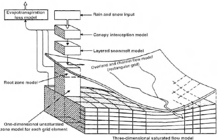
A second strategy has been to reduce the dimensionality of the problem, i.e. to break it down into
smaller pieces. One way to do this has been to treat the unsaturated zone, where flows are predominantly
vertical, as a one-dimensional problem and the saturated zone, where flows are predominantly lateral,
as a two-dimensional problem. This is the approach adopted by the SHE model (Figure 5.3; see, for
example, the work of Abbott
et al.
, 1986a) and some models based on a triangular irregular network
Figure 5.3
Schematic diagram of a grid-based catchment discretisation as in the SHE model (after Refsgaard
and Storm, 1995, with kind permission from Water Resource Publications).