Geoscience Reference
In-Depth Information
Other
Variables
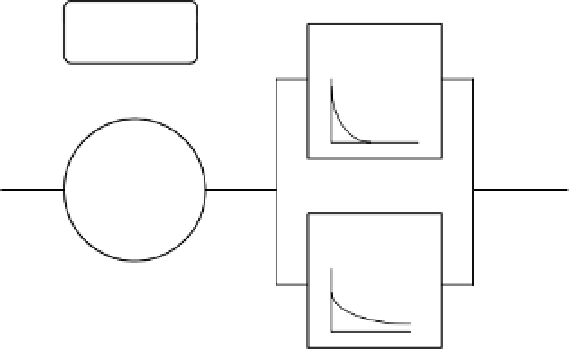
Fast Transfer
Function
Au(t)
u(t)
Nonlinear
Transform
R(t)
Q(t)
Slow Transfer
Function
Bu(t)
Figure 4.4
A parallel transfer function structure and separation of a predicted hydrograph into fast and slow
responses.
Note that these time constants are often referred to as mean residence times for the storage elements
inferred in this type of representation. As is much too often the case in hydrology, this nomenclature is
somewhat confusing since the transfer function as used here refers to the hydrograph response, not to the
actual residence times of water in the system. The response time of the hydrograph and the residence times
of the water in the system are, nearly always, different. Mean residence times for the water in the system
are generally much longer and also tend to vary more as the system wets and dries (see the discussions
of the difference between celerities and velocities in Sections 1.4, 5.5.3 and 11.6). It is worth noting,
however, that this type of transfer function approach has also been used very effectively in modelling
the transport of solutes and pollutants in both surface and subsurface flows. The transfer function, then,
represents the distribution of flow velocities directly. In passing, it is also worth noting this pollution
transport prediction problem is a case where the transfer function model suggests that a classical theory
(here the
advection
-
dispersion
equation) needs some modification before it can reproduce the long tails
seen in tracer experiments and pollution concentration curves (see, for example, the work of Wallis
et al.
,
1989, and Green
et al.
, 1994).
The problem in applying transfer function methods to the rainfall-runoff system is that rainfall is
related to stream discharge in a very nonlinear way. Many years of experience with the use of the
unit hydrograph method in hydrological prediction have shown that storm runoff may be more linearly
related to an “effective” rainfall, but here we wish to avoid any need to carry out any prior separations
of the rainfall and runoff time series since, as discussed in Section 2.2, hydrograph separation is a pretty
desperate analysis technique. However, we can interpret this experience to suggest that it may be possible
to use a linear transfer function model for calculating the time distribution of the total runoff if we can find
an appropriate nonlinear filter on the rainfalls to represent the runoff generation processes. The question
then is how to find the appropriate form of filter.
One way is to simply assume that a certain form is physically reasonable and that constant parameter
values can be found that give a good fit to the data throughout the calibration period. Early work on
linear transfer functions of this type was reported by Jim Dooge (1959) and Eamonn Nash (1960). If
there is truly a linear relationship between the transformed inputs and the measured output data then this
should, in fact, be the case. It is the traditional approach used with unit hydrograph theory where the
transformation from total rainfall to effective rainfall is based on an infiltration equation or a method such
as the
-index method (see Section 2.2). The transfer function based IHACRES model, described below,
also adopts this strategy. However, if an estimate of a transfer function is available for a catchment, we