Time-coordinated optimal power flow for energy service networks - Modelling Distributed Energy Resources in Energy Service Networks - page 94

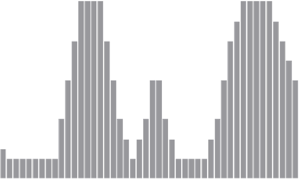
Piecewise constant control profile

1

Values

0.8

0.6

0.4

0.2

0

2 4 6 8 10 12 14 16 18 20 22 24

Time (h)

Figure 5.3 Example of a piecewise constant control variable profile

for complex energy service networks such as the ones modelled in this research,
thus allowing the TCOPF program to reach an optimal solution after a few iterations
independent of network size or topology.
The gPROMS TM CVP-SS solver involves the following steps when implement-
ing its optimisation algorithm [215]:

Starting from the initial time interval, the optimisation algorithm is solved
over the entire time horizon by analysing and deciding the time-variation of
all variables;

●

The optimiser determines when and for how long the control variables should be
active, as well as calculating the values of these control variables;

●

The previous information is used to determine the values of:
-

●

The proposed scalar-valued objective function;

- All the constraints that have to be satisfied by the optimisation algorithm;

Based on the above data, the solver revises the choices it made at the first iteration
and the procedure is repeated until convergence to the optimum is achieved.

●

.
5.1.3 Input data and assumptions of the TCOPF tool
In order to execute the optimisation program, the TCOPF code requires a set of
input data ( i.e. one- or two-dimensional arrays) to process and calculate the optimal
operating values of the energy service networks and their embedded technologies.